High-Accuracy Autonomous Excavation Of Free-Form Shapes
학위논문
한줄 요약 — Dominic Jud의 학위논문은 토질을 몰라도 채우는 힘제어 버킷 사이클부터 12톤 HEAP, 자기변형을 반영하는 0.1 m 지형지도, SQP 이송궤적, 3D cut-fill 계획과 설계 피드백까지 자율 토공의 전 계층을 구축해 cm급 자유형 시공을 보였지만 생산성·GNSS 의존·고가 유압 개조와 예외 복구가 과제로 남는다.
1.연구 배경 및 동기
토질을 미리 알 수 없는 현장에서 설계-측량-굴착을 폐루프로 연결하는 고정밀 자율 토공
건설업의 생산성 향상은 세계 경제 평균보다 느리고, 토공은 여전히 숙련 운전자의 감각에 크게 의존한다. 굴착 자동화는 단순한 팔 궤적 재생이 아니다. 버킷과 토양의 상호작용은 토질·수분·다짐·돌에 따라 달라지고, 한 번의 굴착이 다음 사이클의 지형을 바꾸며, 대형 장비는 제한된 시야와 유압 비선형을 가진다. 따라서 고정 trajectory와 사전 완성 지도만으로는 자연 현장을 안정적으로 정밀 가공하기 어렵다.
이 학위논문은 시뮬레이션의 soil-independent 단일 굴착에서 시작해 세계 최초 자율 보행 굴착기 HEAP, 실차 자유형 trench, 드론 측량과 landscape design이 연결된 3D embankment로 단계적으로 확장된다. 각 단계는 이전 단계가 남긴 현실 문제를 해소한다. 힘 궤적은 토질 모델 의존을 낮추고, HEAP는 정밀 힘·위치 제어와 능동 차체를 제공하며, 지형 매핑은 로봇이 만든 변화를 반영하고, 상위 planner는 수십 m³의 cut과 fill을 설계 오차에 따라 반복한다.
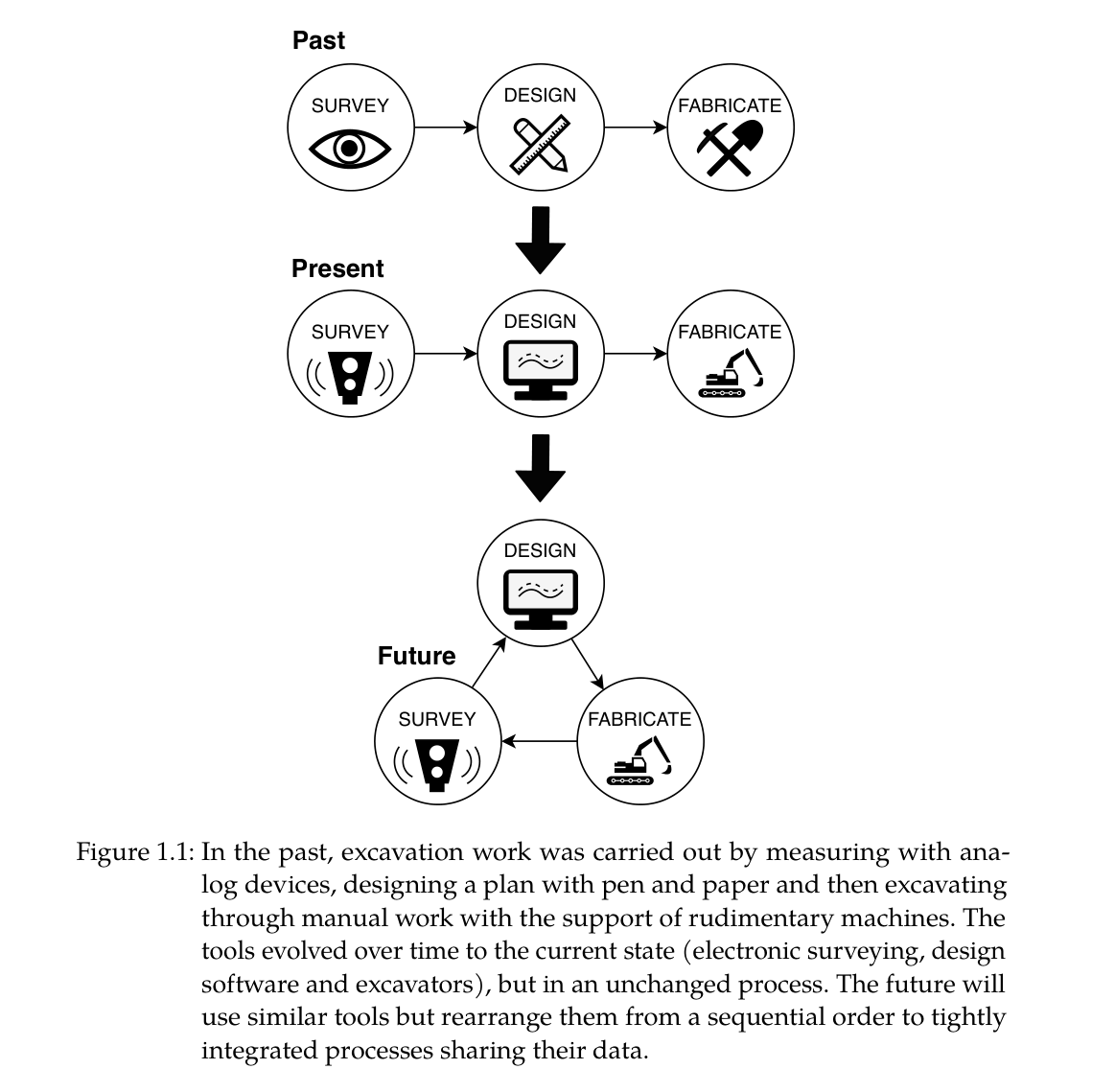
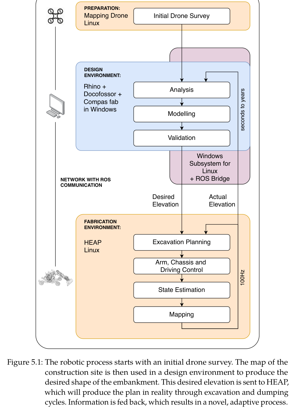
최종 목표는 CAD 형상을 한 번 전달하고 끝내는 자동화가 아니라 survey-design-fabrication의 순환이다. 드론이 현장 전역을 GNSS 좌표로 측량하고 Rhino/Docofossor가 절·성토 균형과 경사를 포함한 목표 지형을 만든다. HEAP가 시공하면서 얻은 elevation map은 설계에 되돌아가며, S형 제방 실험에서는 공정 약 3분의 2 지점에 실제 cut-fill 불균형을 반영해 설계를 수정했다.
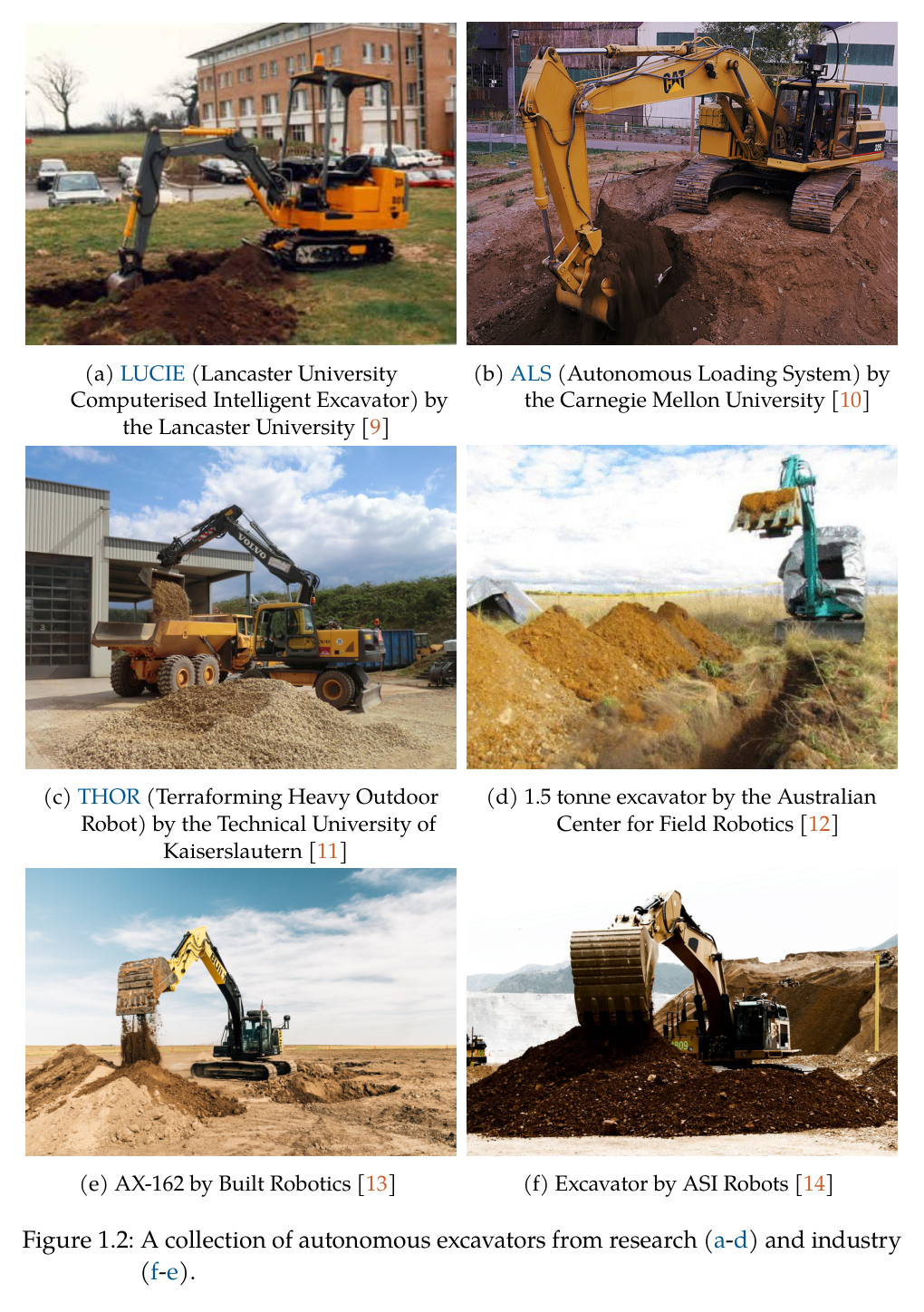
원문 Figure 1.1 · PDF p.19 — Figure 1.1: In the past, excavation work was carried out by measuring with ana- log devices, designing a plan with pen and paper and then excavating through manual work with the support of rudimentary machines. The tools evolved over time to the current state (electronic surveying, design software and excavators), but in an unchanged process. The future will use similar tools but rearrange them from a sequential order to tightly integrated processes sharing their data.원문 Figure 1.2 · PDF p.21 — Figure 1.2: A collection of autonomous excavators from research (a-d) and industry (f-e).
선행 연구의 한계
position trajectory 기반 굴착은 토질 저항이 달라지면 bucket fill과 경로 추종이 동시에 무너지고 과도한 힘 또는 빈 버킷을 만들 수 있다.
기존 자율굴착 연구는 평면·단순 trench, 고정형 장비, 사전 알려진 토질이나 simulation에 집중해 자유곡면과 이동형 대형 현장 검증이 부족했다.
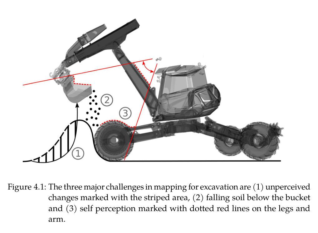
일반 elevation mapping은 정적 환경을 가정해 가려진 굴착부, 공중에서 떨어지는 토사, 로봇 자체 점군 때문에 로봇이 만든 변화를 잘못 기록한다.
기존 landscape workflow는 survey-설계-시공이 한 번씩 순차 진행돼 현장에서 발견한 재료·토량·오차가 설계에 즉시 환류되지 않는다.
상용 굴착기는 밸브 데드존·낮은 force-control 대역폭·차체 흔들림 때문에 cm급 말단 제어를 위한 하드웨어와 전신 안정화가 부족하다.
이 연구의 기여
penetrate-drag-close 힘/토크 궤적과 버킷 충전량 기반 상태 전환으로 토질 물성 입력 없이 한 번의 굴착을 수행하는 방법을 제안했다.
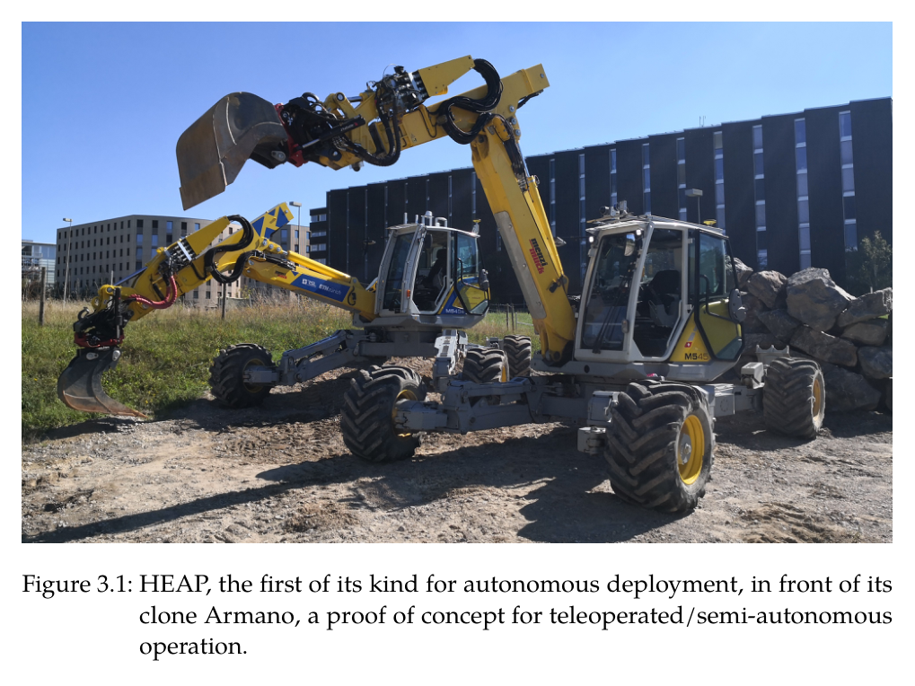
센싱·세 가지 팔 구동·상태추정·능동 차체·계층형 팔 제어가 통합된 12톤 HEAP를 구축해 자율 토공의 실차 기반을 만들었다.
LiDAR exteroception과 버킷 edge proprioception, 낙토·self filter를 융합한 굴착용 0.1 m elevation map 및 SDF-SQP 충돌회피 이송계획을 개발했다.
단일 사이클 cut/fill planner를 3D 진행면·오차 blob·driving path로 확장하고 드론 측량·Docofossor 설계·HEAP fabrication의 양방향 landscape workflow를 구현했다.
자유형 trench에서 평균 0.024–0.027 m, 30 m³ S형 embankment 전체 0.056 m, 두 면 corner embankment 0.032 m의 실차 정밀도를 입증했다.
2.방법론 및 시스템 구성
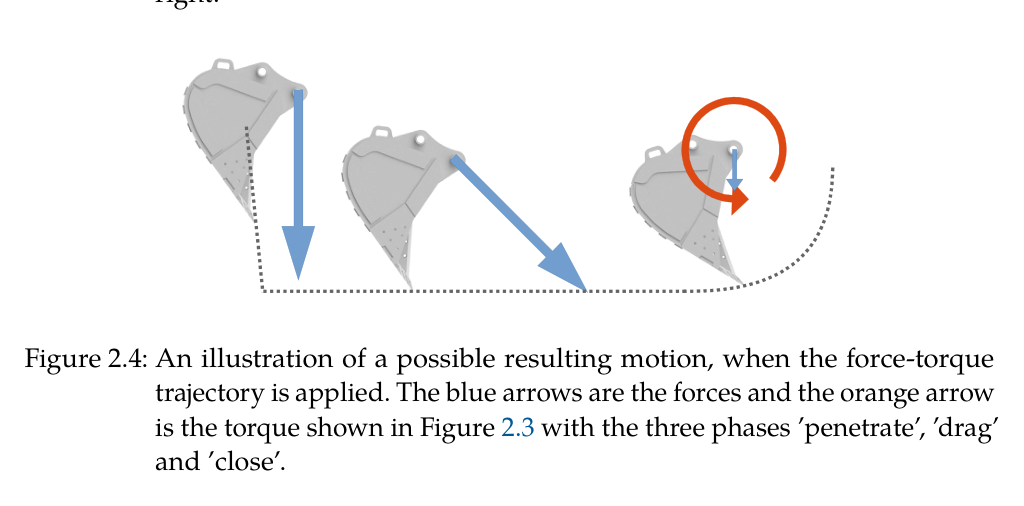
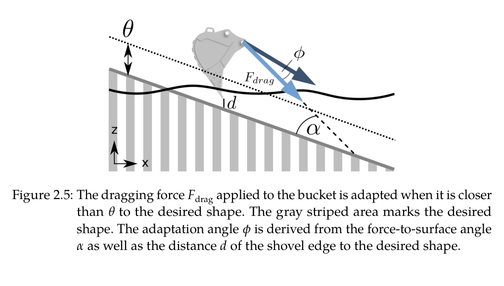
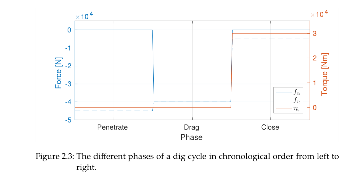
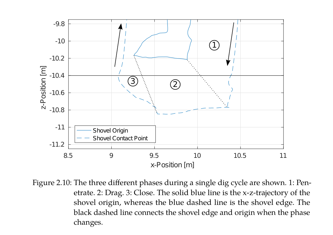
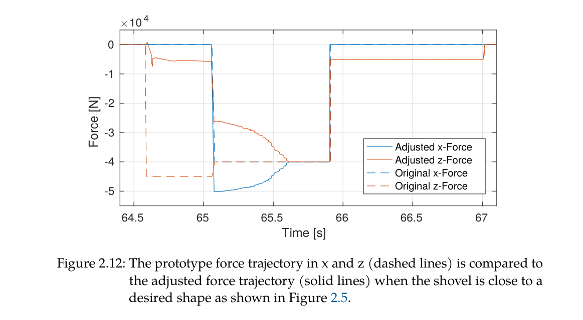
하위 굴착 동작은 bucket task-space force/torque를 penetration, drag, close 세 phase로 정의한다. penetration은 아래쪽 힘으로 지면에 들어가고, drag는 굴착방향과 아래방향 힘을 주되 목표면 근처에서는 힘 크기를 줄여 stick-slip을 만드는 대신 힘 벡터를 회전한다. bucket edge가 쓸고 간 지형으로 예상 충전 부피를 적산해 용량을 넘으면 close로 전환하며, close에서는 bucket torque와 작은 하향 힘으로 유출을 억제한다.
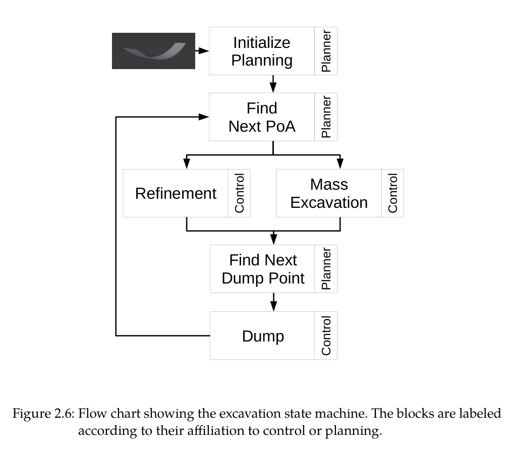
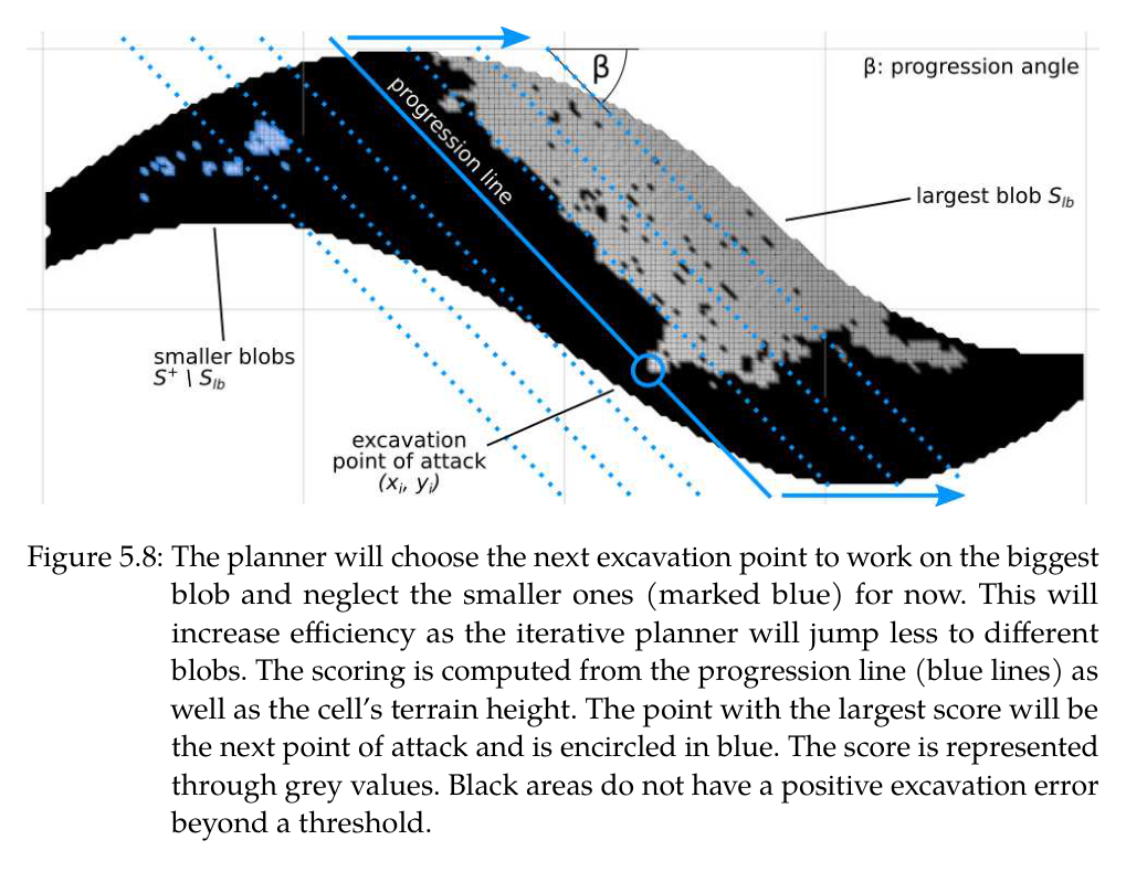
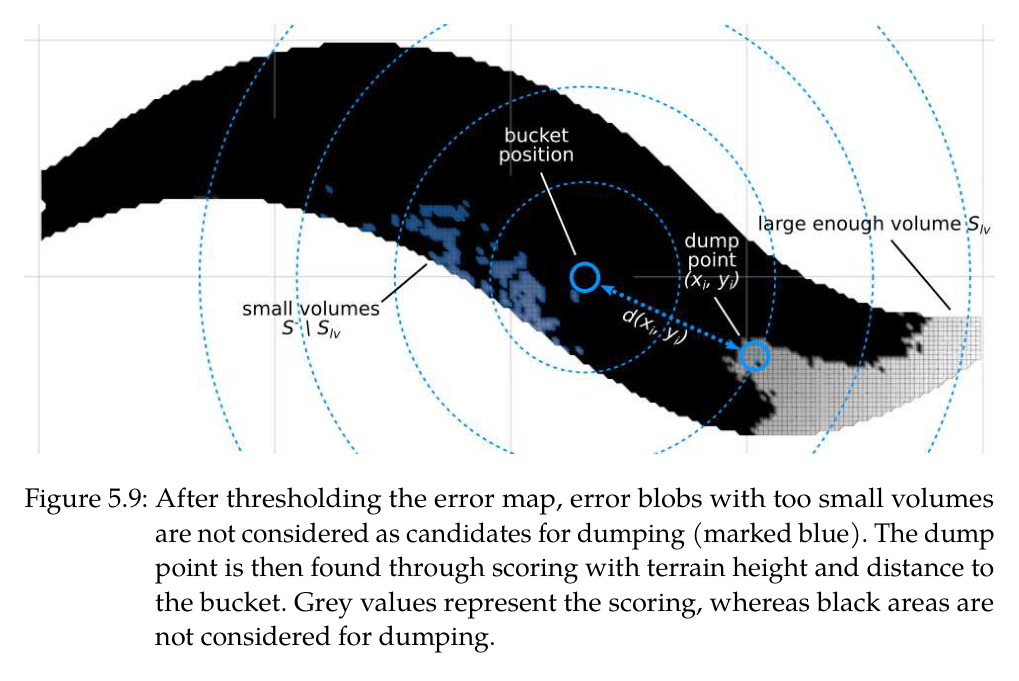
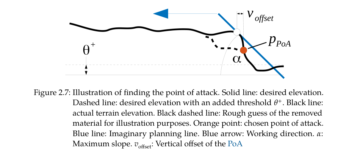
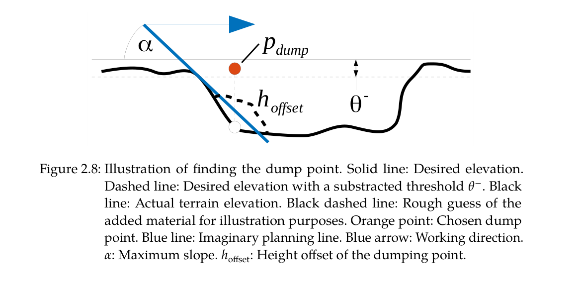
다중 사이클 planner는 실제 elevation과 desired elevation의 cell error를 계산해 threshold보다 높은 cut cell에서 point of attack을, 낮은 fill cell에서 dump point를 찾는다. 거리와 높이, 허용 slope를 score에 넣어 높은 벽 밑을 파는 위험과 긴 이동을 피한다. 큰 오차에서는 힘제어 mass excavation을 사용하고 목표면에 가까워지면 inverse-kinematic grading으로 전환한다.
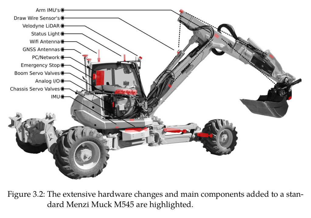
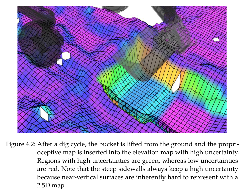
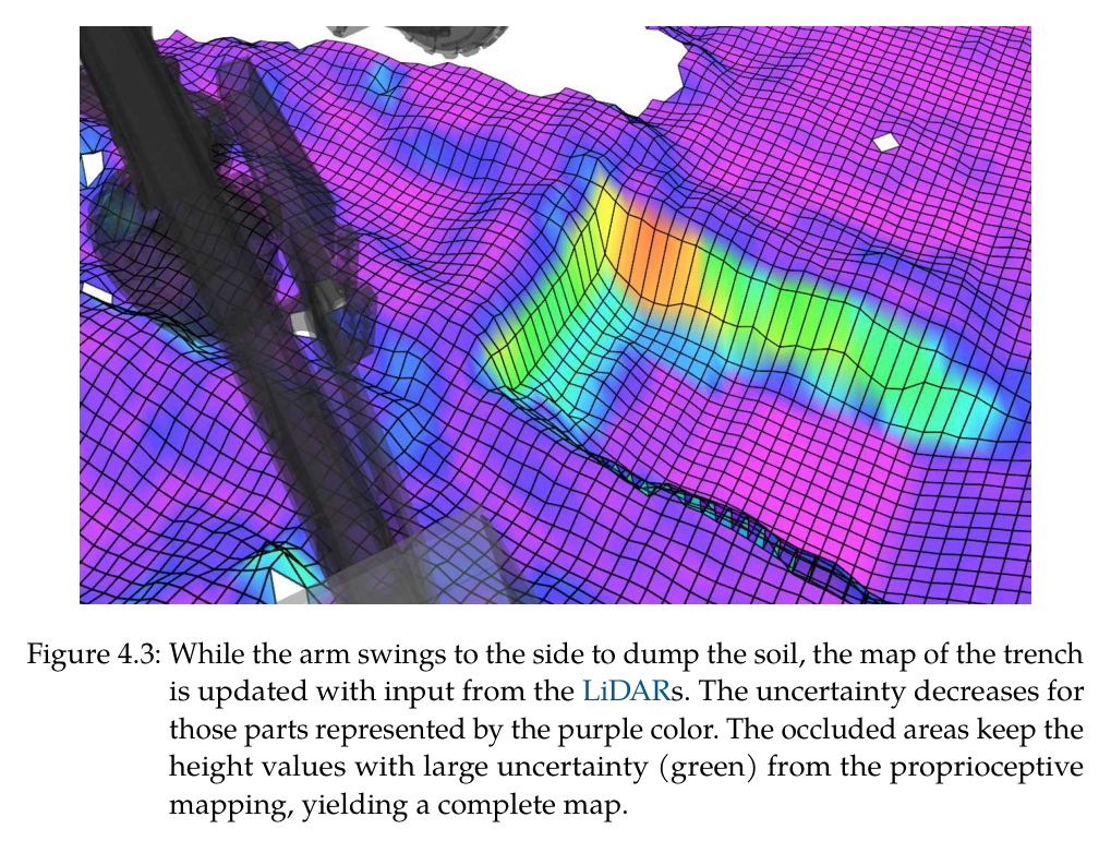
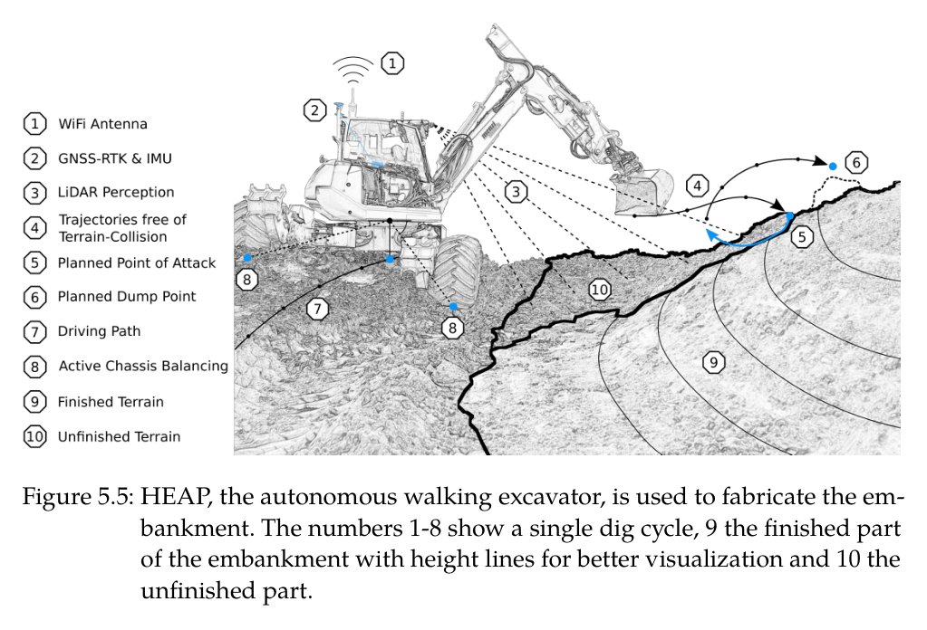
실차 HEAP는 두 VLP-16, GNSS-RTK·IMU, 실린더 encoder·압력센서와 능동 wheel-leg chassis를 사용한다. mapping은 LiDAR 점군에 self filter와 bucket 하부 falling-soil box를 적용하고, LiDAR가 가린 굴착부에는 measured bucket-edge sweep를 높은 불확실도로 삽입한다. 캐빈이 dump 쪽으로 회전하면 새 LiDAR 관측이 그 영역의 불확실도를 다시 낮춘다.
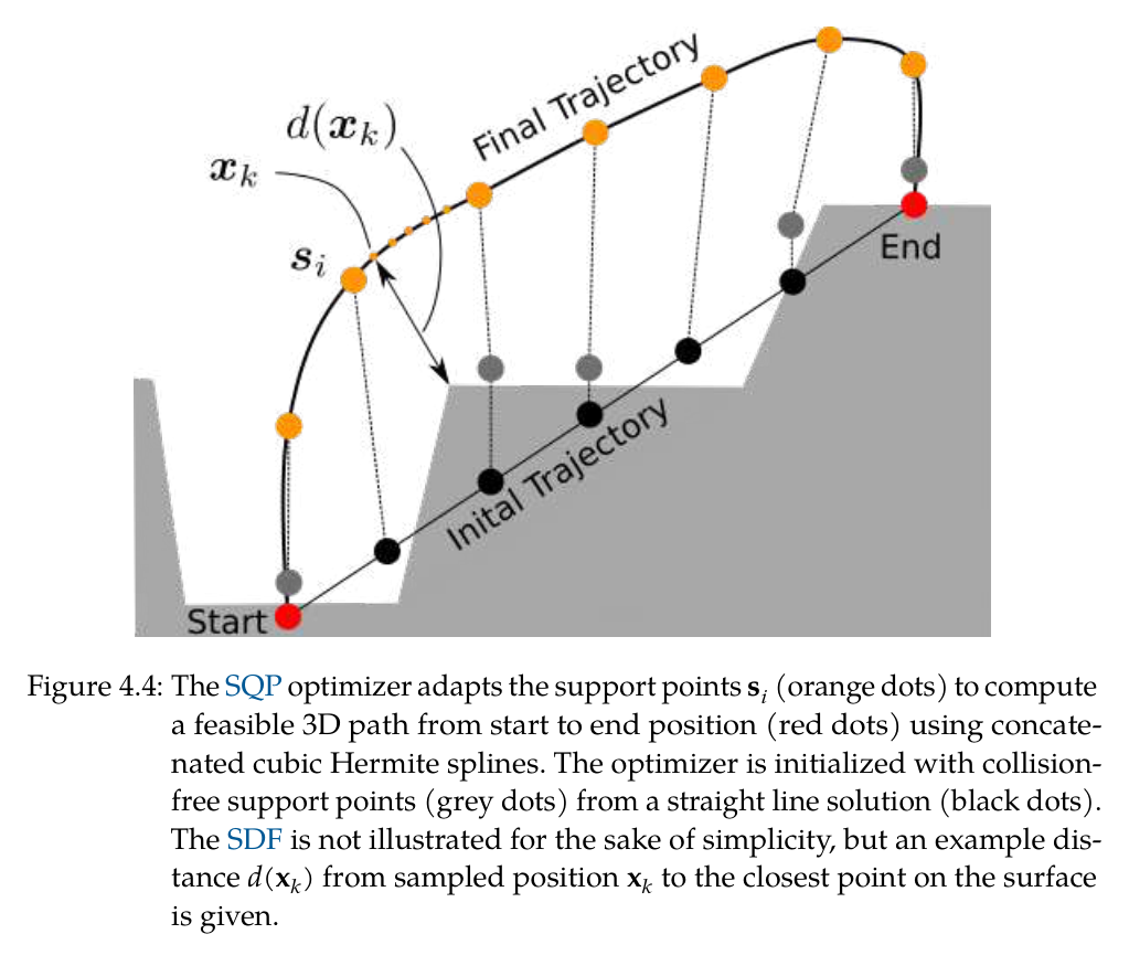
공중 bucket 이송은 2.5D map에서 만든 3D signed distance field와 cubic Hermite spline을 사용한다. 직선 support point를 충돌 밖으로 초기화하고 SQP가 경로 길이, SDF collision, support-point 간격 regularization을 동시에 줄인다. 자기충돌은 계층형 arm controller가 국소적으로 피하며, 가득 찬 bucket은 orientation을 position보다 높은 우선순위로 둬 토사 유출을 막는다.
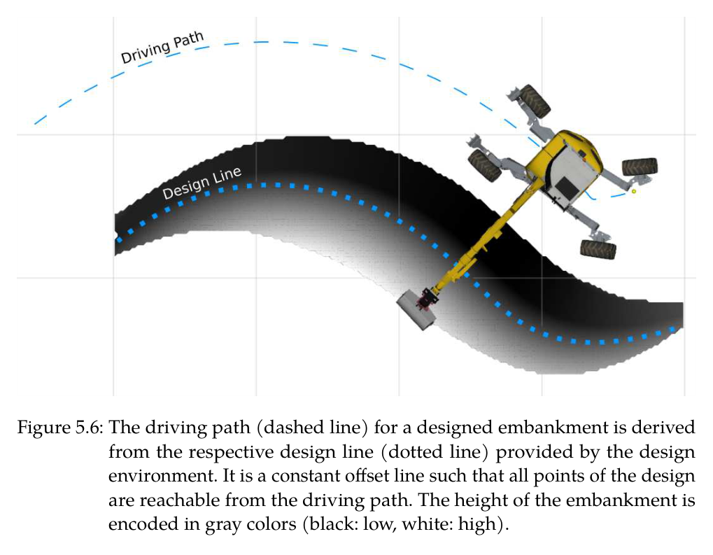
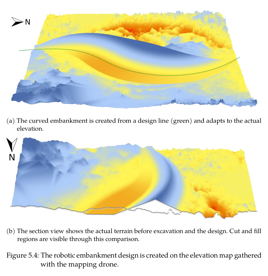
embankment 단계에서는 DJI M210 RTK의 Ouster OS1로 전역 지도를 만들고 Rhino/Docofossor가 cut-fill 균형, swell, 최대 경사를 포함한 목표 elevation과 design line을 생성한다. HEAP는 design line의 offset을 driving path로 삼고 진행 plane과 최대 error blob으로 다음 cut을, 거리·고도와 최소 오차부피로 dump를 정한다. 시공 map을 설계로 돌려보내 필요하면 형상을 수정한다.
처리 파이프라인
1
초기 현장 측량과 좌표 통일
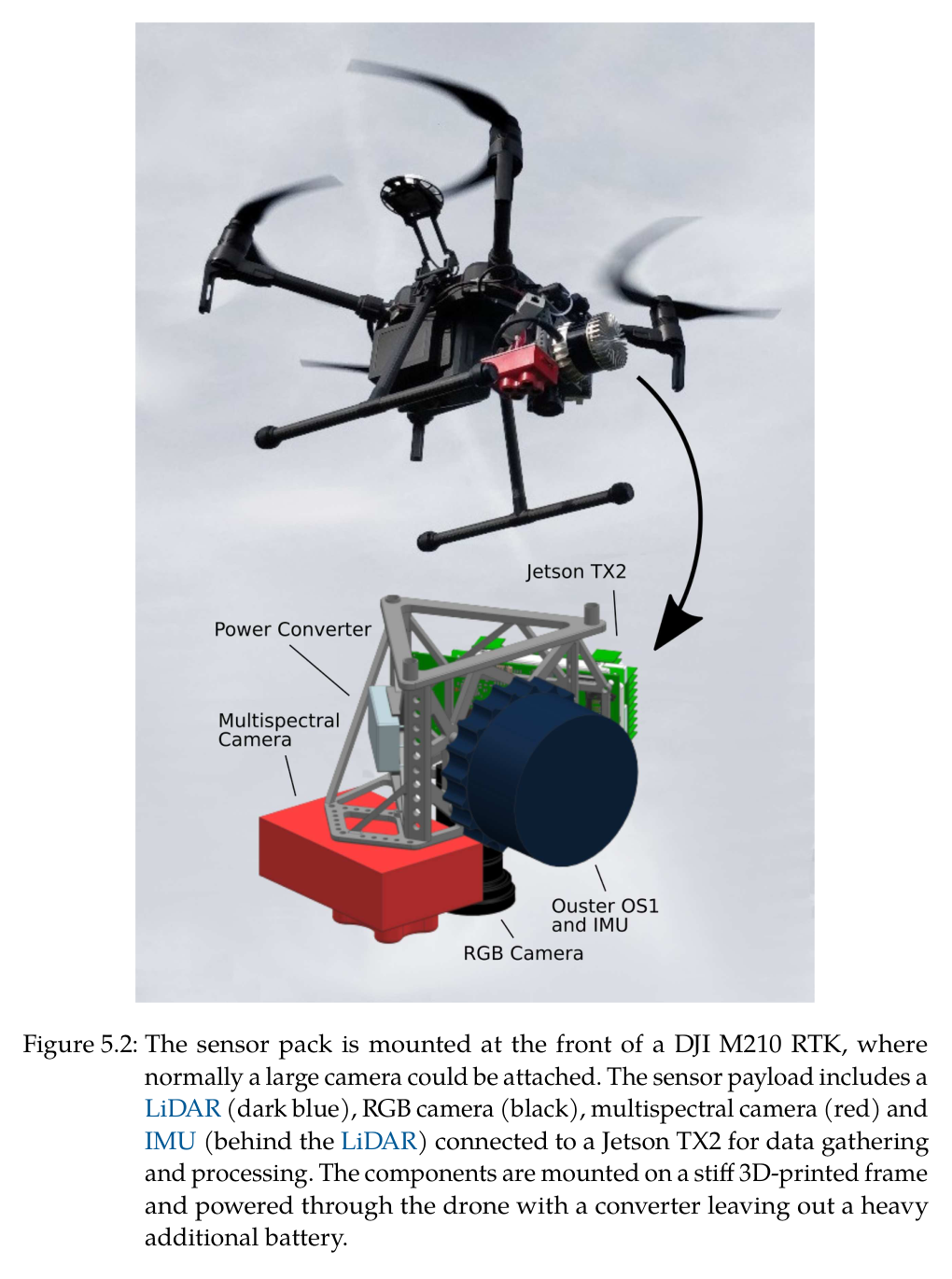
DJI M210 RTK에 64-line Ouster OS1, IMU, Jetson TX2를 싣고 수동 비행으로 LiDAR packet과 drone state를 기록한다. lidar_align으로 외부변환·시간 offset을 맞추고 3D 점군을 2.5D elevation map으로 바꾼다. drone과 HEAP가 모두 GNSS-RTK 세계좌표를 사용해 설계와 실차가 정렬된다.
2
terrain-aware landscape design
Rhino의 Docofossor에서 design line과 단면을 정의하고 초기 terrain과 비교해 cut/fill volume을 균형화한다. swell factor와 maximum slope를 검토하고 ROS bridge를 통해 desired elevation과 design line을 HEAP에 전송한다.
3
굴착 중 폐루프 elevation mapping
HEAP 지붕의 직교 LiDAR가 0.1 m grid를 갱신하고 robot mesh와 가득 찬 bucket 아래 낙토 점을 제거한다. 가려진 굴착부는 bucket edge trajectory로 즉시 대체한 뒤 후속 LiDAR 관측으로 uncertainty를 낮춘다.
4
cut point와 chassis 위치 선택
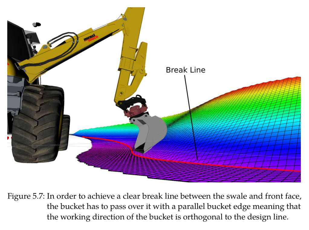
actual-desired error threshold와 largest blob mask로 실제 작업할 pile을 고른다. 3D progression plane score가 높은 부분부터 진행시키고, bucket edge가 design break line과 평행하도록 arm working direction을 design line에 직교시킨다. reach 밖이면 pure-pursuit로 offset driving path를 이동한다.
5
SDF-SQP 접근 궤적
current bucket pose와 PoA 또는 dump point 사이에 Hermite spline을 만들고 elevation SDF로 지면 distance·gradient를 얻는다. SQP가 support point를 이동시켜 충돌 clearance, path length, 간격 regularity를 만족한다.
6
토질 독립 force-controlled dig
접촉을 확보한 뒤 penetration force, drag force, bucket close torque를 순차 실행한다. 목표면 근처에서는 drag force direction을 표면 방향으로 회전하고, bucket swept volume이 capacity에 이르면 close 및 이송으로 넘어간다.
7
fill point와 정밀 grading
negative error map에서 작은 blob을 제외하고 가까우며 낮은 dump cell을 선택한다. full bucket을 투하해 약간 과성토한 뒤 다음 cut/IK grading으로 오차를 제거하며, 목표면 근처나 고접촉력에서는 force와 position mode를 상태기계가 전환한다.
8
시공-설계 feedback
HEAP의 current elevation을 design environment로 반환해 토량·재료·형상 차이를 평가한다. S형 실험처럼 진행 중 설계를 다시 계산해 남은 cut과 fill을 균형화하고 수정 elevation을 다음 사이클에 사용한다.
원문 수식과 의미
point-of-attack 선택
threshold보다 높은 cut cell 중 terrain height와 excavator까지의 거리/허용 slope를 결합해, 안정한 진행 방향에서 다음 굴착 시작점을 고른다.
SDF spline 총비용
Hermite spline 표본의 경로 길이, 지형까지 거리가 epsilon 이내일 때의 collision penalty, support-point 간격 표준편차를 가중합해 SQP로 최소화한다.
task-space 굴착 force의 joint 변환
원하는 bucket force/torque를 Jacobian으로 joint torque에 매핑하고 Coriolis·중력과 점성·정지마찰을 보상해 실차 servo valve 명령을 만든다.
3D embankment cut score
largest error blob 안에서 현재 높이와 각도 beta의 진행 plane을 결합해 상부 토사를 먼저 제거하고 좌우 시공 순서를 안정화한다.
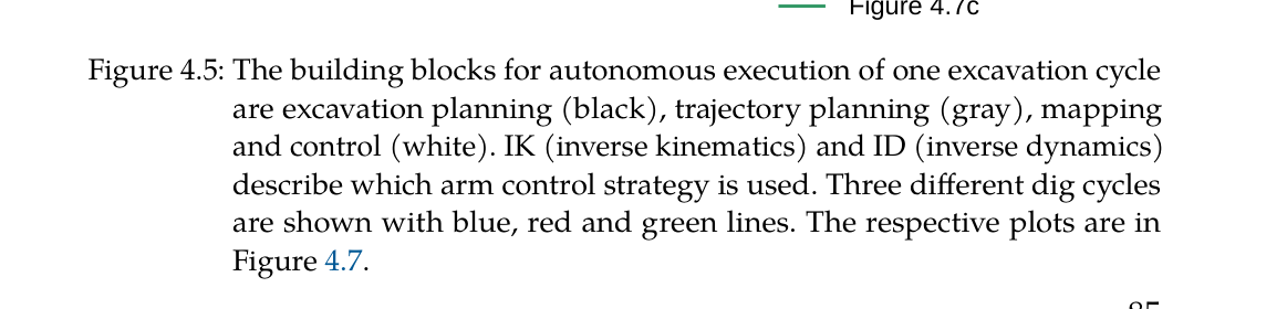
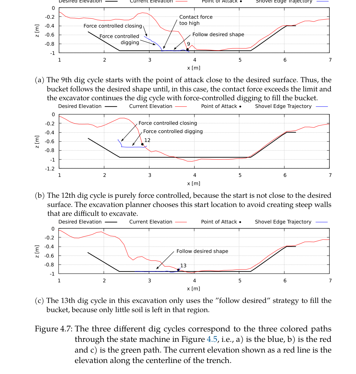
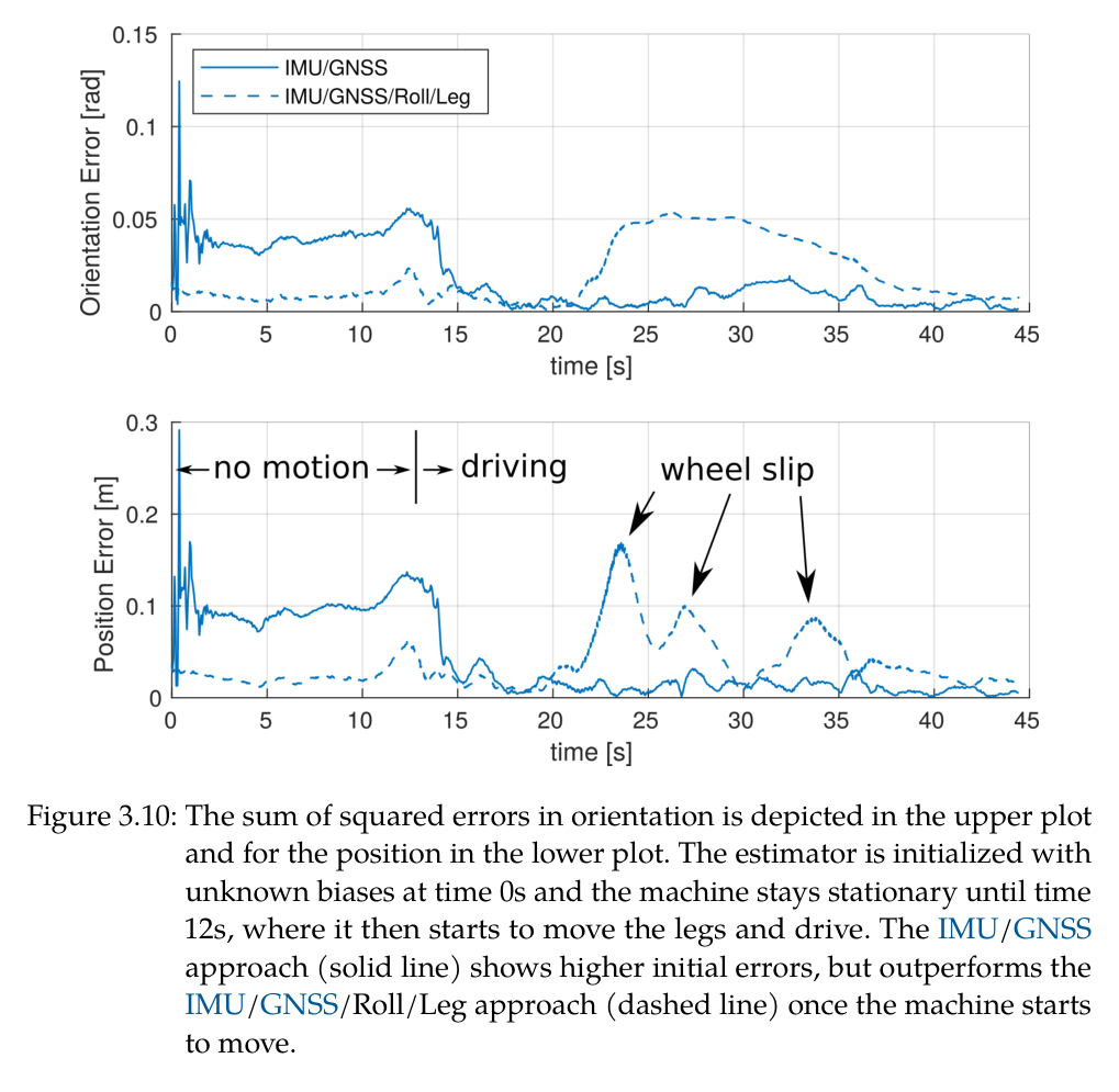
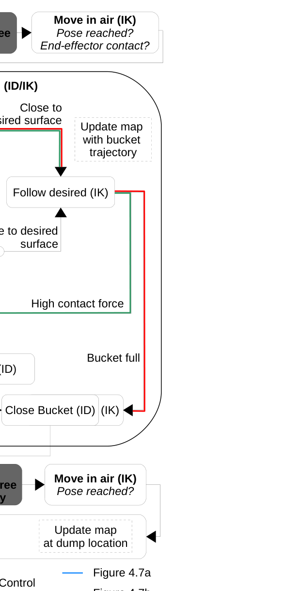
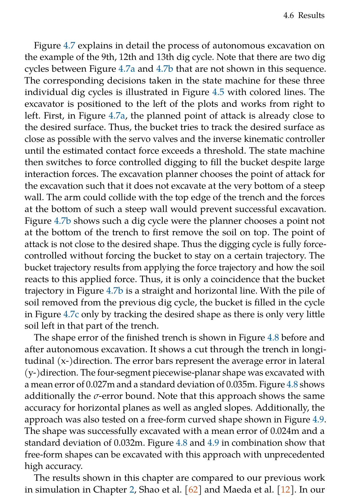
원문 Figure 2.4 · PDF p.40 — Figure 2.4: An illustration of a possible resulting motion, when the force-torque trajectory is applied. The blue arrows are the forces and the orange arrow is the torque shown in Figure 2.3 with the three phases ’penetrate’, ’drag’ and ’close’.원문 Figure 2.6 · PDF p.45 — Figure 2.6: Flow chart showing the excavation state machine. The blocks are labeled according to their affiliation to control or planning.원문 Figure 4.1 · PDF p.94 — Figure 4.1: The three major challenges in mapping for excavation are (1) unperceived changes marked with the striped area, (2) falling soil below the bucket and (3) self perception marked with dotted red lines on the legs and arm.원문 Figure 4.4 · PDF p.98 — Figure 4.4: The SQP optimizer adapts the support points 𝐬𝑖(orange dots) to compute a feasible 3D path from start to end position (red dots) using concate- nated cubic Hermite splines. The optimizer is initialized with collision- free support points (grey dots) from a straight line solution (black dots). The SDF is not illustrated for the sake of simplicity, but an example dis- tance 𝑑(𝐱𝑘) from sampled position 𝐱𝑘to the closest point on the surface is given.원문 Figure 4.5 · PDF p.101 — Figure 4.5: The building blocks for autonomous execution of one excavation cycle are excavation planning (black), trajectory planning (gray), mapping and control (white). IK (inverse kinematics) and ID (inverse dynamics) describe which arm control strategy is used. Three different dig cycles are shown with blue, red and green lines. The respective plots are in Figure 4.7.원문 Figure 5.1 · PDF p.111 — Figure 5.1: The robotic process starts with an initial drone survey. The map of the construction site is then used in a design environment to produce the desired shape of the embankment. This desired elevation is sent to HEAP, which will produce the plan in reality through excavation and dumping cycles. Information is fed back, which results in a novel, adaptive process.원문 Figure 5.6 · PDF p.119 — Figure 5.6: The driving path (dashed line) for a designed embankment is derived from the respective design line (dotted line) provided by the design environment. It is a constant offset line such that all points of the design are reachable from the driving path. The height of the embankment is encoded in gray colors (black: low, white: high).원문 Figure 5.8 · PDF p.121 — Figure 5.8: The planner will choose the next excavation point to work on the biggest blob and neglect the smaller ones (marked blue) for now. This will increase efficiency as the iterative planner will jump less to different blobs. The scoring is computed from the progression line (blue lines) as well as the cell’s terrain height. The point with the largest score will be the next point of attack and is encircled in blue. The score is represented through grey values. Black areas do not have a positive excavation error beyond a threshold.원문 Figure 5.9 · PDF p.123 — Figure 5.9: After thresholding the error map, error blobs with too small volumes are not considered as candidates for dumping (marked blue). The dump point is then found through scoring with terrain height and distance to the bucket. Grey values represent the scoring, whereas black areas are not considered for dumping.
3.핵심 기술
토질을 직접 추정하지 않는 force/torque dig trajectory
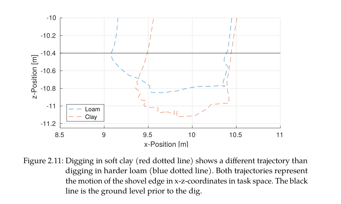
시스템은 soil parameter를 식별해 resistive-force model을 푸는 대신 bucket이 지면과 상호작용하는 힘과 단계 전환을 설계한다. 같은 command에서도 단단한 토양은 penetration이 얕아 drag가 길어지고, 부드러운 토양은 깊게 들어가 짧은 drag와 회전형 close로 이어진다. 즉 토질 차이가 제어 실패가 아니라 동작 형태의 자연스러운 변화로 나타난다.
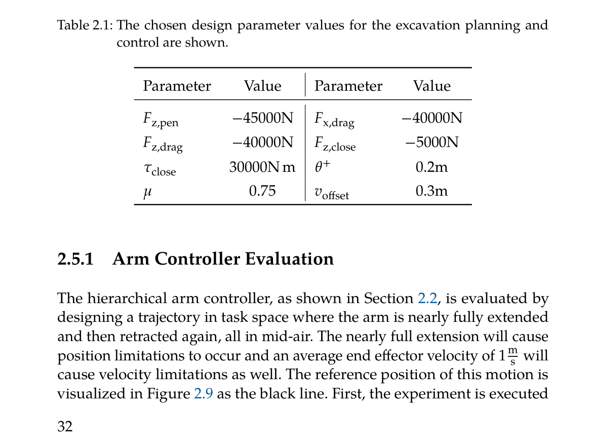
시뮬레이션 설정은 penetration -45 kN, drag x/z 각각 -40 kN, close 하향 -5 kN과 bucket torque 30 kNm를 사용했다. loam과 clay 실험에서 clay는 50% 더 깊게 penetration되고 drag 거리는 50% 짧아졌음에도 별도 soil-dependent trajectory를 주지 않았다. force vector rotation은 목표면 근처에서 magnitude 감쇠가 만드는 stick-slip을 피한다.
penetrate-drag-close 세 단계와 bucket swept-volume 종료조건
목표면 거리 0.2 m 안에서 drag force 방향을 회전
토질 물성 입력 없이 soil interaction이 phase 길이를 조절
actuator-aware hierarchical arm control과 안정한 HEAP
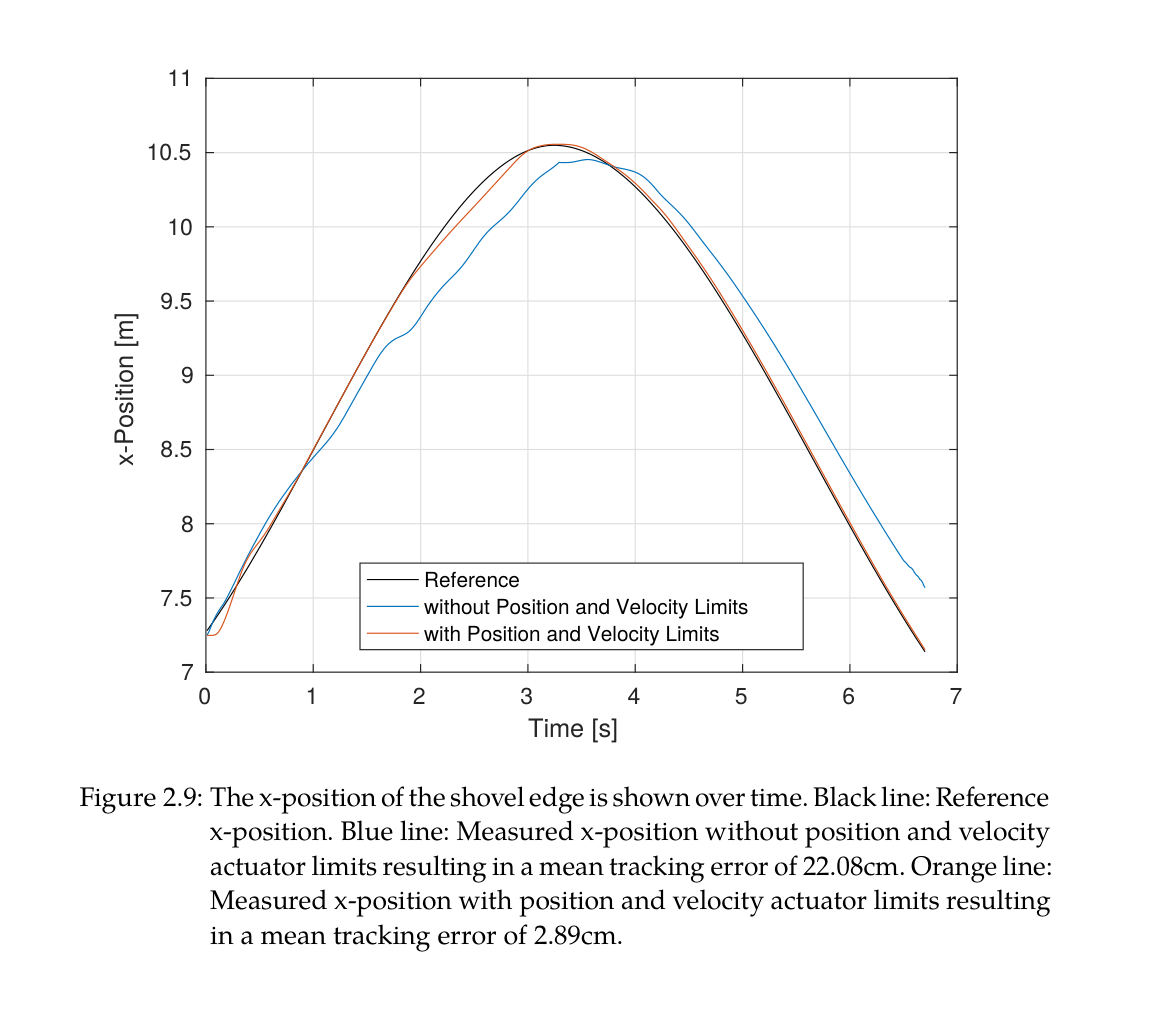
계층형 최적화는 end-effector 과제뿐 아니라 joint position·velocity·cylinder force·pump flow·self-collision 제약을 높은 우선순위에 둔다. 팔이 거의 완전히 펴지는 1 m/s 공중 궤적에서 actuator limit를 무시하면 평균 22.08 cm가 되었지만, 제약을 켜면 redundancy를 이용해 2.89 cm로 줄었다. 이는 알고리즘적 한계처리가 정밀도에 직접 영향을 준다는 절제 결과다.
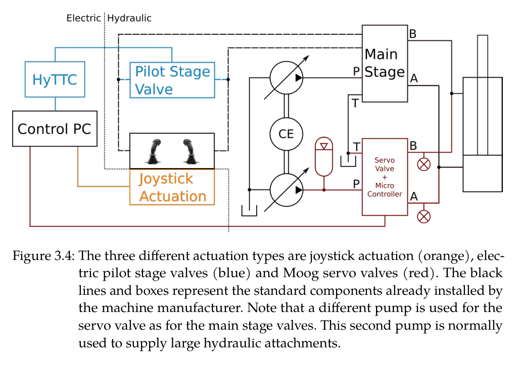
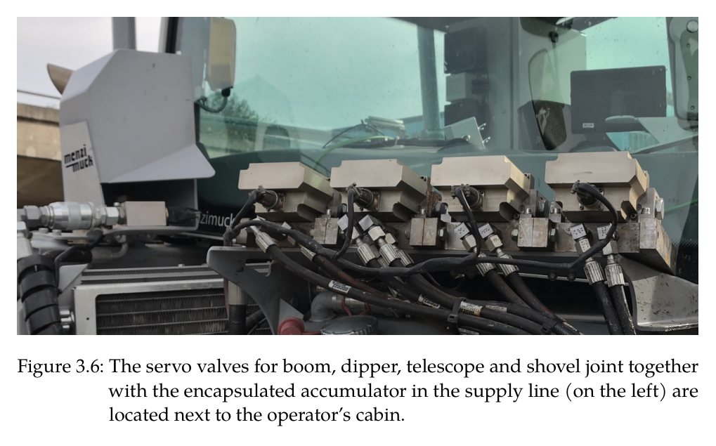
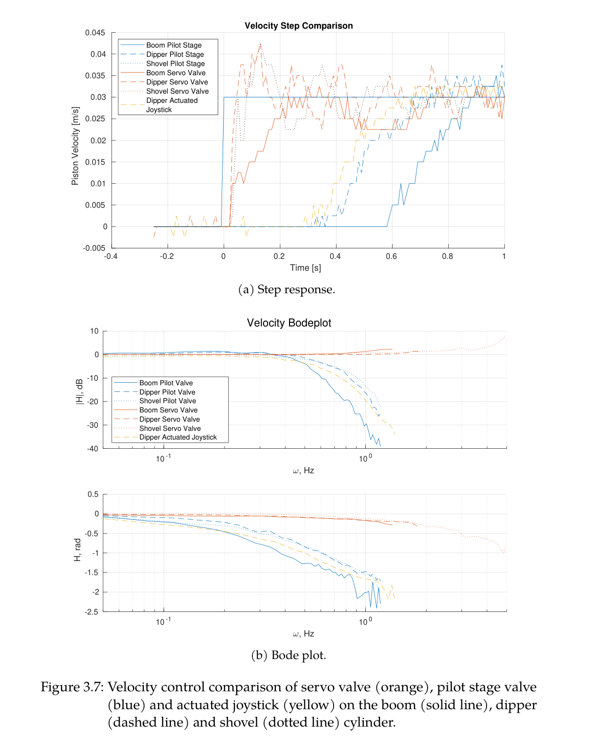
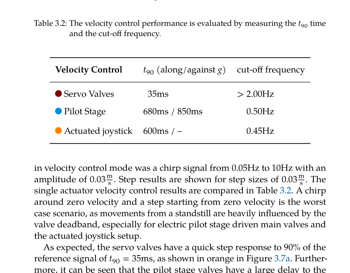
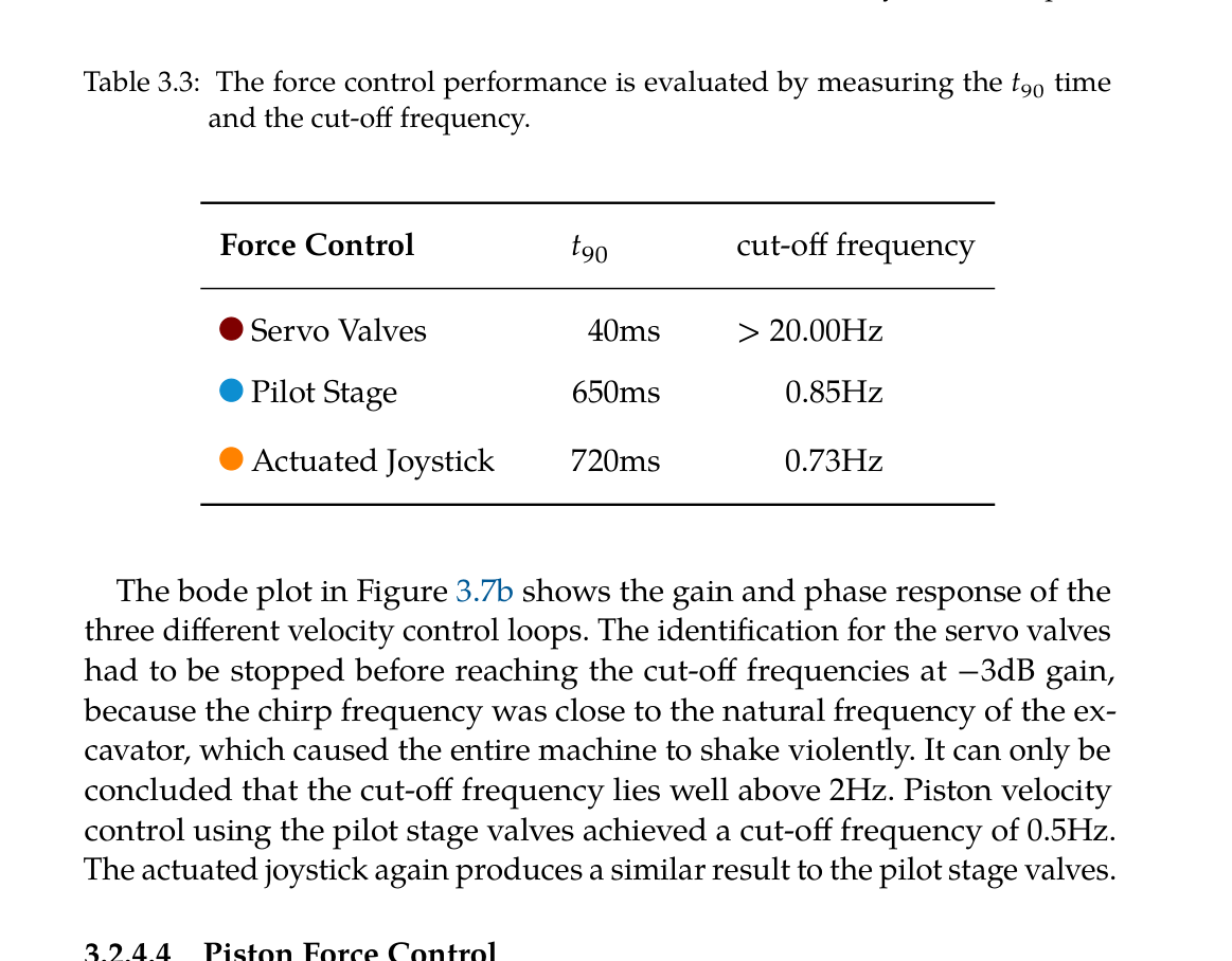
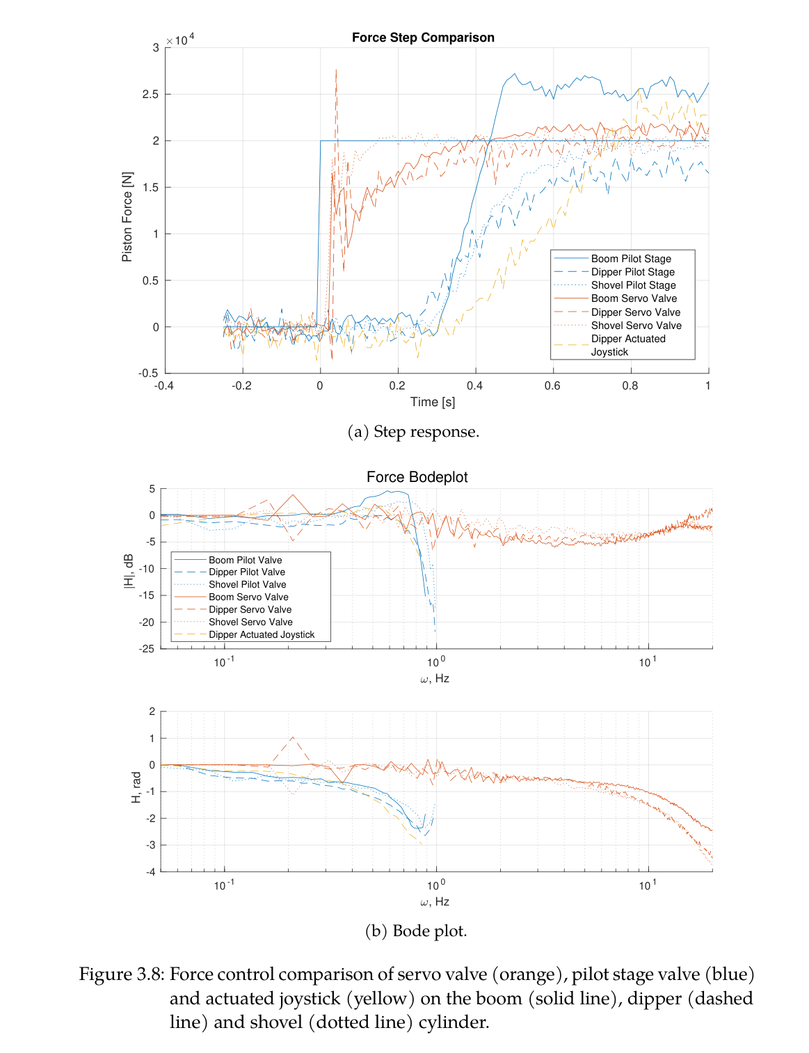
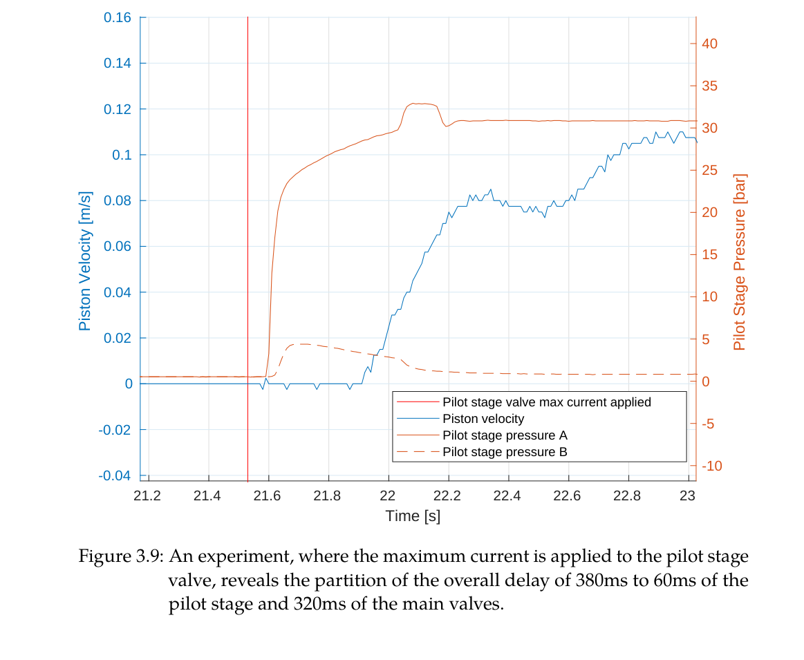
실차에서는 공중 이송은 유량이 큰 pilot-stage main valve, 지면 접촉은 빠른 고압 servo valve를 사용한다. 능동 chassis는 네 wheel 접촉과 base 자세를 유지해 무거운 arm의 가감속이 만드는 rocking을 줄인다. 고정밀 trench는 force controller만이 아니라 안정한 세계좌표와 ground contact를 제공하는 플랫폼 수준 설계의 결과다.
actuator limit 반영으로 mean tracking error 87% 감소
servo valve는 접촉 force, pilot valve는 빠른 공중 이동에 역할 분담
능동 chassis가 모든 wheel 접촉을 유지해 end-effector 기준 안정화
로봇이 만든 변화를 아는 proprioceptive-exteroceptive map
굴착 순간의 새 표면은 남은 pile에 가려 LiDAR가 보지 못할 수 있다. 그러나 로봇은 bucket edge가 지나간 위치를 알고 있으므로 그 sweep를 높은 uncertainty의 임시 지형으로 삽입한다. 이후 cabin이 dump 방향으로 회전해 시야가 열리면 LiDAR가 실제 높이로 빠르게 교체한다. map hole을 기다리지 않고 다음 cycle을 계획할 수 있다는 점이 단순 정적 mapping과 다르다.
가득 찬 bucket 아래 이동 box는 낙하 중인 soil point가 허공의 벽으로 적산되는 것을 막고, multi-mesh self filter는 arm·leg 점을 제거한다. 0.1 m grid는 1.5 m bucket 폭보다 15배 작아 자유형 surface 계획과 cm급 최종 오차를 지원하면서도 전체 작업장 연산량을 제한한다.
bucket-edge sweep를 occluded excavation spot에 높은 uncertainty로 삽입
bucket 하부 falling-soil box와 multi-mesh robot self filter
GNSS georeferenced 0.1 m elevation map
충돌 없는 자유형 trench 상태기계
한 cycle은 PoA 선택, SDF-SQP 공중 접근, contact 확보, force dig 또는 IK surface following, close, dump point 선택, collision-free 이송, map update로 구성된다. 시작점이 목표면에 가까우면 position grading을 하고, 예상 contact force가 커지면 force dig로 바꾸며, bucket이 다리·차체에 가까워지면 조기에 종료한다. 실차 uncertainty를 mode switching과 안전조건으로 흡수한다.
Hermite spline의 collision weight를 길이보다 크게 하면 지면에서 거의 수직으로 이탈·접근해 bucket이 edge를 긁을 위험을 낮춘다. arm self-collision은 controller, terrain collision은 planner로 분리해 서로 다른 시간척도에서 안전을 다룬다.
force mass excavation와 IK refinement를 contact·surface distance로 전환
SDF가 지면 아래 시작점도 부호 있는 거리로 표현
bucket full 또는 imminent self-collision에서 dig 종료
drone-design-HEAP의 3D cut/fill feedback
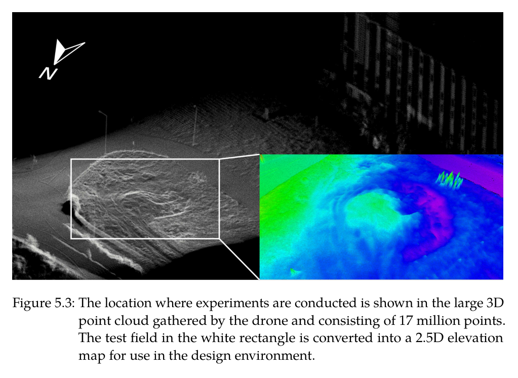
DJI M210 RTK의 1.72 kg payload에는 380 g, 64-line Ouster OS1과 Jetson TX2가 실렸고, 최종 point cloud는 1,700만 점이었다. Docofossor는 이 지형 위에서 material-neutral embankment를 설계하고 cut/fill, swell, slope를 검토한다. 설계선의 offset driving path는 HEAP reach와 구조물 보존을 함께 만족한다.
3D cut planner는 가장 큰 positive-error blob에서 progression plane score가 큰 셀을, dump planner는 negative-error blob 중 가까운 낮은 셀을 고른다. 0.1 m³보다 작은 fill blob은 full bucket 투하가 오히려 오차를 키우므로 제외한다. 로봇이 partial bucket dump를 못한다는 하드웨어 한계를 상위 계획의 공간 threshold로 변환한 사례다.
drone 17 million-point survey와 GNSS 좌표 공유
largest cut blob과 3D progression plane으로 장거리 재방문 감소
fill error volume <0.1 m³ 제외 후 과성토-재굴착 방식
원문 Figure 2.5 · PDF p.43 — Figure 2.5: The dragging force 𝐹drag applied to the bucket is adapted when it is closer than 𝜃to the desired shape. The gray striped area marks the desired shape. The adaptation angle 𝜙is derived from the force-to-surface angle 𝛼as well as the distance 𝑑of the shovel edge to the desired shape.원문 Figure 2.9 · PDF p.49 — Figure 2.9: The x-position of the shovel edge is shown over time. Black line: Reference x-position. Blue line: Measured x-position without position and velocity actuator limits resulting in a mean tracking error of 22.08cm. Orange line: Measured x-position with position and velocity actuator limits resulting in a mean tracking error of 2.89cm.원문 Figure 3.2 · PDF p.59 — Figure 3.2: The extensive hardware changes and main components added to a stan- dard Menzi Muck M545 are highlighted.원문 Figure 4.2 · PDF p.95 — Figure 4.2: After a dig cycle, the bucket is lifted from the ground and the propri- oceptive map is inserted into the elevation map with high uncertainty. Regions with high uncertainties are green, whereas low uncertainties are red. Note that the steep sidewalls always keep a high uncertainty because near-vertical surfaces are inherently hard to represent with a 2.5D map.원문 Figure 4.3 · PDF p.96 — Figure 4.3: While the arm swings to the side to dump the soil, the map of the trench is updated with input from the LiDARs. The uncertainty decreases for those parts represented by the purple color. The occluded areas keep the height values with large uncertainty (green) from the proprioceptive mapping, yielding a complete map.원문 Figure 5.2 · PDF p.113 — Figure 5.2: The sensor pack is mounted at the front of a DJI M210 RTK, where normally a large camera could be attached. The sensor payload includes a LiDAR (dark blue), RGB camera (black), multispectral camera (red) and IMU (behind the LiDAR) connected to a Jetson TX2 for data gathering and processing. The components are mounted on a stiff 3D-printed frame and powered through the drone with a converter leaving out a heavy additional battery.원문 Figure 5.5 · PDF p.117 — Figure 5.5: HEAP, the autonomous walking excavator, is used to fabricate the em- bankment. The numbers 1-8 show a single dig cycle, 9 the finished part of the embankment with height lines for better visualization and 10 the unfinished part.
4.실험 결과
실험 환경·장비·데이터
Vortex soil mechanics simulation과 0.2 m elevation grid, 0.580 m³ bucket model
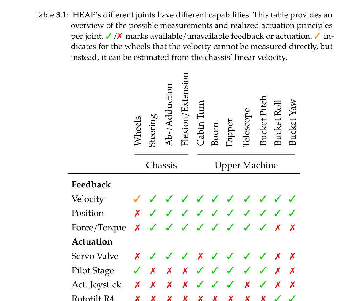
12톤 Menzi Muck M545 기반 HEAP, 31자유도, 두 VLP-16, GNSS-RTK·IMU·실린더/압력센서, servo/pilot hydraulic actuation
실차 free-form trench용 폭 1.5 m toothless bucket와 0.1 m robot-centric elevation map
실외 clay-rich 시험장, 집중호우 후 33.7° S형 제방과 두 면 corner 제방
실험 프로토콜
시뮬레이션에서 actuator position/velocity limit task를 끄고 켠 동일 1 m/s arm 궤적의 mean shovel-edge error를 비교했다.
loam과 clay에서 같은 force parameters로 단일 dig를 수행해 penetration·drag 형태와 bucket fill의 토질 적응을 관찰했다.
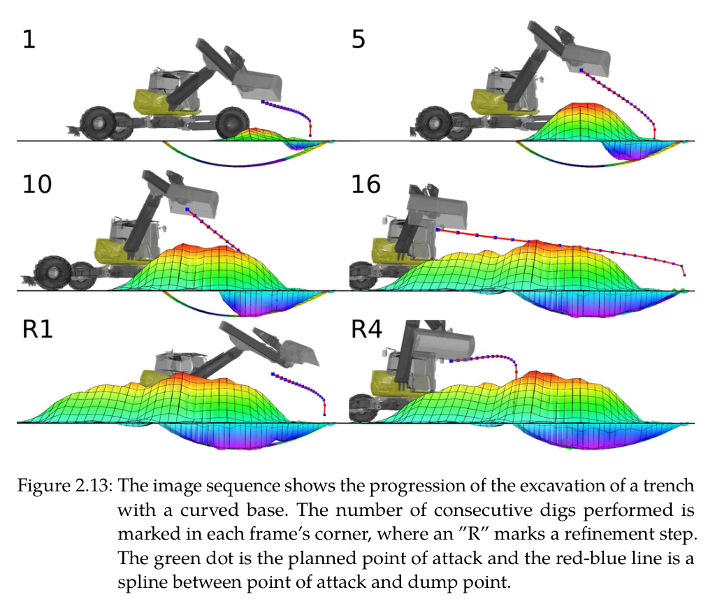
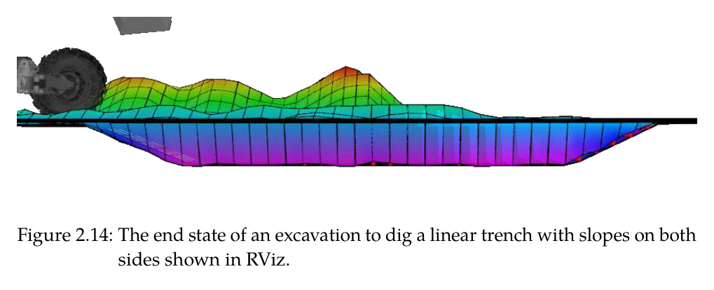
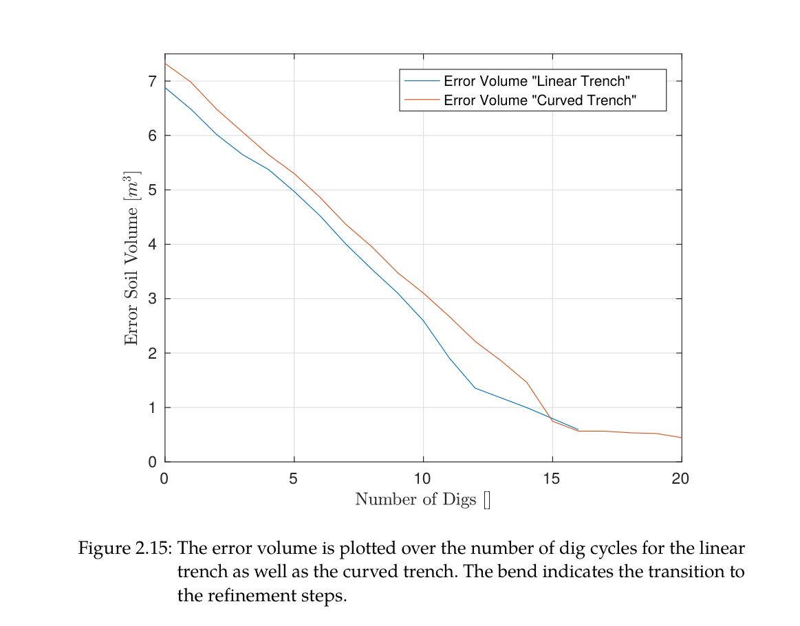
곡면 trench는 16회 force dig 뒤 4회 refinement를 수행했고, 사면을 가진 linear trench도 elevation error와 error-volume 감소로 평가했다.
실차에서 수평·경사 linear segment와 curved free-form target을 excavation state machine으로 만들고 desired-surface normal 방향의 cell error를 계산했다.
S형 embankment는 drone survey→설계→HEAP fabrication을 수행하고 공정 약 2/3 시점에 remaining cut/fill을 재균형화해 설계를 수정했다.
두 면 corner 제방은 구조를 사람이 한 차례 무너뜨린 후 autonomy가 excess·missing soil을 다시 찾아 복구하도록 했다.
비교 기준
arm controller 절제: actuator position/velocity limit 과제 사용 대 미사용
trench 비교: thesis simulation 0.035/0.044 m, Shao et al. <0.1 m, Maeda et al. 0.025 m와 실차 free-form 결과 비교
Maeda 접근은 exteroceptive terrain map 없이 bucket motion으로 surface를 추정하므로 자유형 지형 인식 범위가 다름
S형 제방 내부 비교: 완만한 concave 구간 대 flat-edge bucket이 접근하기 어려운 tight convex 구간
작업 모드: force-controlled rough excavation 대 IK position refinement
평가 지표
shovel-edge mean tracking error와 actuator-limit 감소율
desired elevation까지의 mean cell error와 표준편차, normal-direction error map
dig당 compacted/swelled volume과 bucket capacity
cut·fill volume, swell factor, 기계 운전시간, 설계 adaptation 시점
embankment 전체·부분·corner surface error와 slope
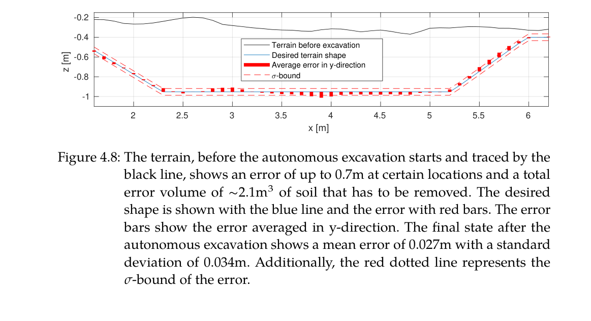
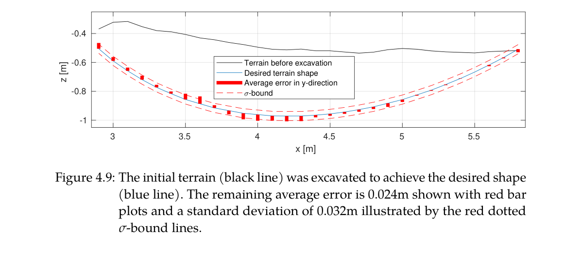
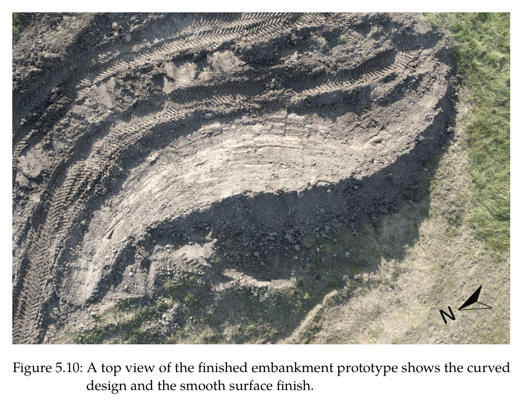
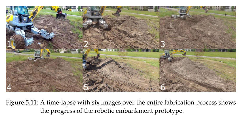
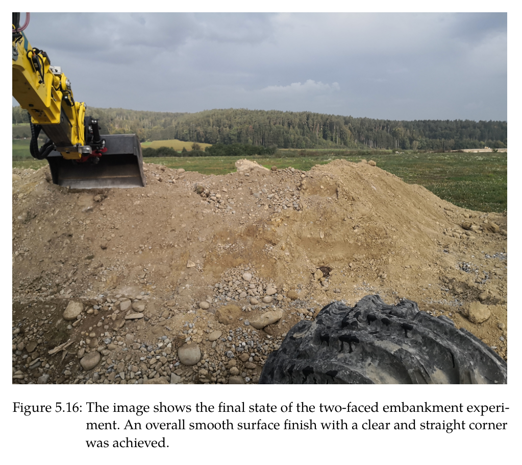
원문 Figure 2.13 · PDF p.53 — Figure 2.13: The image sequence shows the progression of the excavation of a trench with a curved base. The number of consecutive digs performed is marked in each frame’s corner, where an ”R” marks a refinement step. The green dot is the planned point of attack and the red-blue line is a spline between point of attack and dump point.원문 Figure 2.14 · PDF p.53 — Figure 2.14: The end state of an excavation to dig a linear trench with slopes on both sides shown in RViz.원문 Figure 4.7 · PDF p.104 — Figure 4.7: The three different dig cycles correspond to the three colored paths through the state machine in Figure 4.5, i.e., a) is the blue, b) is the red and c) is the green path. The current elevation shown as a red line is the elevation along the centerline of the trench.원문 Figure 4.8 · PDF p.106 — Figure 4.8: The terrain, before the autonomous excavation starts and traced by the black line, shows an error of up to 0.7m at certain locations and a total error volume of ∼2.1m3 of soil that has to be removed. The desired shape is shown with the blue line and the error with red bars. The error bars show the error averaged in y-direction. The final state after the autonomous excavation shows a mean error of 0.027m with a standard deviation of 0.034m. Additionally, the red dotted line represents the 𝜎-bound of the error.원문 Figure 4.9 · PDF p.106 — Figure 4.9: The initial terrain (black line) was excavated to achieve the desired shape (blue line). The remaining average error is 0.024m shown with red bar plots and a standard deviation of 0.032m illustrated by the red dotted 𝜎-bound lines.원문 Figure 5.10 · PDF p.125 — Figure 5.10: A top view of the finished embankment prototype shows the curved design and the smooth surface finish.원문 Figure 5.11 · PDF p.125 — Figure 5.11: A time-lapse with six images over the entire fabrication process shows the progress of the robotic embankment prototype.원문 Figure 5.16 · PDF p.130 — Figure 5.16: The image shows the final state of the two-faced embankment experi- ment. An overall smooth surface finish with a clear and straight corner was achieved.
핵심 결과 해석
시뮬레이션에서 actuator 한계를 모르는 arm controller는 평균 22.08 cm 오차였고, position·velocity limit를 계층 과제로 넣자 2.89 cm로 87% 감소했다. 같은 force trajectory는 토질 파라미터 없이 loam과 clay에서 다르게 적응했고, 한 cycle이 평균 0.440 m³ compacted soil을 제거했다. loam swell 1.4를 적용하면 0.616 m³로 0.580 m³ bucket 명목용량보다 많아 상부에 쌓일 정도의 fill을 보였다. 곡면 trench는 16 rough digs와 4 refinements 뒤 3.47 cm, 사면 linear trench는 4.41 cm 평균 높이오차였다.
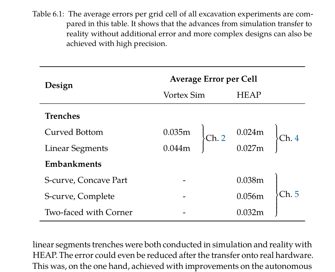
실차 free-form trench에서는 horizontal과 angled linear segment를 함께 평가해 평균 0.027 m, 표준편차 약 0.035/0.034 m를 얻었고, curved target은 평균 0.024 m와 표준편차 0.032 m였다. 1.5 m toothless bucket이라는 거친 도구로도 centimeter-scale profile이 가능했다. 핵심은 LiDAR만으로 보이는 표면을 기다리지 않고 bucket-edge map update, force dig, IK refinement를 cycle마다 반복한 데 있다.
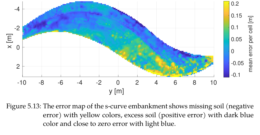
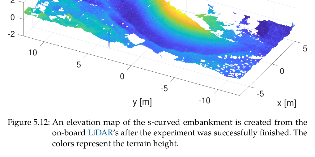
최종 S형 embankment는 slope 33.7°, 설계 displacement 30 m³였으며 총 6시간 동안 30.60 m³를 cut하고 32.20 m³를 fill했다. 사용 swell factor는 1.05였다. 완만한 concave 구간은 mean cell error 0.038 m로 trench와 유사했지만, flat bucket으로 tight convex curvature에 접근하기 어려워 전체는 0.056 m로 커졌다. 이 failure pattern은 양의 오차가 cut 영역, 음의 오차가 fill 영역과 대응했다.
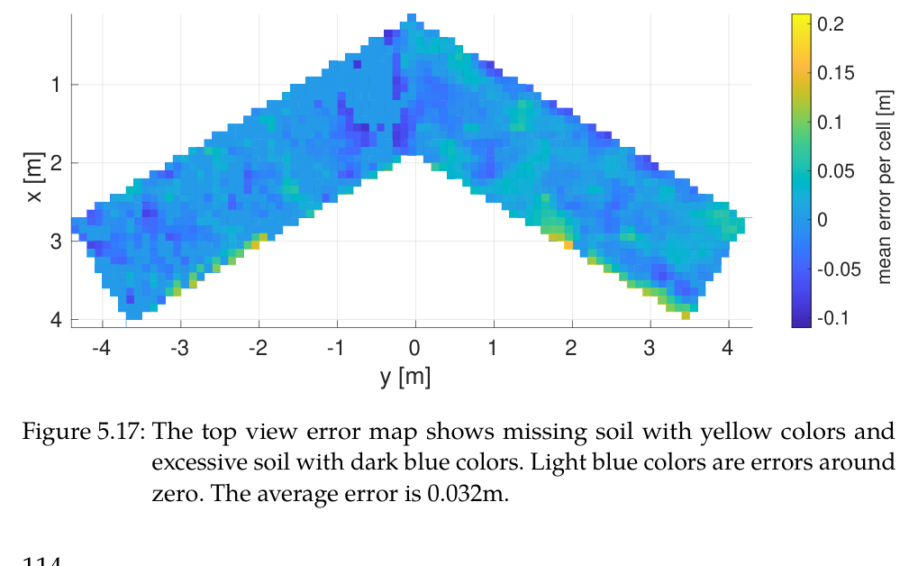
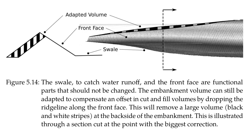
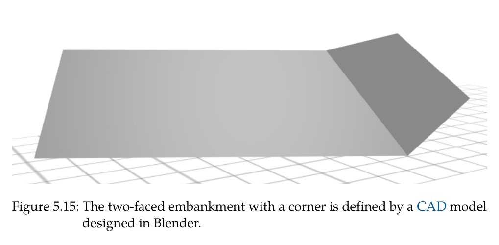
공정 약 3분의 2 지점에서 초기 survey/design의 토량 추정이 실제와 맞지 않자 design을 재계산해 cut/fill을 다시 균형화했다. 이는 fabrication feedback이 단순 monitoring을 넘어 남은 목표 geometry를 실제로 변경한 증거다. 두 면과 명확한 corner를 가진 별도 embankment는 mean error 0.032 m였고, 사람이 한 차례 무너뜨린 뒤에도 시스템이 error map을 바탕으로 자율 복구했다.
논문 전체의 정량표는 simulation에서 reality로 옮길 때 오차가 악화되지 않았음을 강조한다. 그러나 human operator와 동일 형상의 생산속도·연료·버킷당 cycle time을 통제 비교하지 않았고, Level 4 분류에서도 캐빈 감독자는 남았다. 따라서 성과는 고정밀·통합 autonomy의 proof이지, 이미 인간보다 빠른 상용 토공이라는 주장은 아니다.
정량 결과
평가 항목
정량 결과
조건·맥락
원문 근거
actuator-aware arm tracking
22.08 cm→2.89 cm, 87% 감소
1 m/s 공중 궤적, position/velocity limit task off/on
PDF p.49
simulation curved trench
평균 3.47 cm
16 force dig+4 refinement
PDF p.52
simulation linear slope trench
평균 4.41 cm
사면 두 개를 포함한 목표 geometry
PDF p.52
평균 dig volume
0.440 m³ compacted=0.616 m³ at swell 1.4
0.580 m³ bucket 명목용량과 비교
PDF p.54
실차 linear free-form trench
평균 0.027 m, 표준편차 0.035 m
horizontal 및 angled segment
PDF p.105
실차 curved free-form trench
평균 0.024 m, 표준편차 0.032 m
1.5 m toothless bucket
PDF p.106
drone survey
17 million points
DJI M210 RTK와 Ouster OS1 현장 전역 점군
PDF p.114
S형 제방 설계
33.7°, 30 m³
강우 후 clay-rich soil에 설정한 slope와 displacement
PDF p.124
S형 제방 생산량
6 h, cut 30.60 m³, fill 32.20 m³, swell 1.05
전체 autonomous machine operation
PDF p.126
S형 제방 surface error
concave 0.038 m, 전체 0.056 m
tight convex 구간이 전체 오차를 증가
PDF p.127
두 면 corner 제방
평균 0.032 m
manual destruction 뒤 autonomous rebuild 포함
PDF p.130
작은 fill blob threshold
<0.1 m³ 제외
full bucket 투하가 오차를 키우는 영역 회피
PDF p.123
실패 사례와 경계조건
S형 제방의 남쪽 tight convex 곡률은 flat-edge bucket이 접근하기 어려워 concave 0.038 m보다 전체 오차를 0.056 m로 높였다.
초기 설계의 cut/fill 양이 실제 시공과 맞지 않아 약 2/3 진행 뒤 재설계가 필요했으며, 고정 open-loop design이면 토량 불균형이 남았을 것이다.
full bucket의 일부만 정량 투하할 수 없어 0.1 m³보다 작은 fill error blob은 의도적으로 무시해 정확도를 일부 희생했다.
굴착 시작점이 목표면에 가까워도 돌·뿌리 때문에 IK grading force가 커지면 force-control로 후퇴해야 했다.
LiDAR vertical surface와 occlusion은 2.5D map uncertainty를 높였고, bucket proprioception이 없는 순수 exteroceptive map은 blind digging 변화를 놓쳤다.
원문 Figure 5.13 · PDF p.127 — Figure 5.13: The error map of the s-curve embankment shows missing soil (negative error) with yellow colors, excess soil (positive error) with dark blue color and close to zero error with light blue.원문 Figure 5.17 · PDF p.130 — Figure 5.17: The top view error map shows missing soil with yellow colors and excessive soil with dark blue colors. Light blue colors are errors around zero. The average error is 0.032m.
5.한계 및 향후 연구
현재 한계
HEAP의 생산성은 숙련 인간보다 낮고, 논문은 같은 지형을 대상으로 한 cycle time·연료·비용의 통제 비교를 제공하지 않는다.
절대 위치와 drone-design-HEAP 좌표 연결이 GNSS-RTK에 크게 의존해 차폐·다중경로 환경에서 cm급 정밀도 유지가 어렵다.
정밀 force control에 고가 servo valve와 대규모 hydraulic retrofit이 필요하며 off-the-shelf excavator는 같은 controller를 바로 실행할 수 없다.
2.5D elevation map은 overhang·수직면을 직접 표현하기 어렵고, bucket edge sweep도 실제 soil collapse와 hidden cavity를 완전하게 측정하지 않는다.
계획은 한 dig cycle 앞을 보는 반복 heuristic이어서 전체 driving·dig·dump 순서를 장기 최적화하지 못하고 작은 오차에 재방문할 수 있다.
Level 4 prototype에서도 사람이 캐빈에서 감독했고 예상 밖 장애물·센서고장·작업자 진입을 일반적으로 복구하는 safety system은 범위 밖이다.
향후 연구
학습 기반 hydraulic control로 pilot/main valve의 deadband와 비선형을 보상해 servo valve 수와 retrofit 비용을 줄이고 속도를 높인다.
높은 수준의 excavation policy를 학습해 여러 cycle의 cut·dump·driving 순서를 공동 최적화하고 인간 생산성에 가까운 작업전략을 얻는다.
visual odometry와 추가 localization을 GNSS-IMU에 융합해 위성 신호가 불안정한 urban·산림 현장으로 확장한다.
multispectral·RGB·force 정보를 map과 design feedback에 넣어 soil composition, moisture, compactability에 따라 slope와 공정 순서를 바꾼다.
여러 excavator·drone·운반장비의 작업영역과 토량을 조정하는 multi-machine planning으로 현장 규모와 생산성을 높인다.
partial bucket dumping, tool change 또는 curved grading attachment를 개발해 작은 fill error와 tight convex surface의 기하 한계를 줄인다.
6.한마디로 정리
핵심 방법은?
힘기반 단일 dig, actuator-aware HEAP 제어, proprioceptive-exteroceptive mapping, SDF-SQP 이송, 3D cut/fill planner와 design feedback을 전 계층으로 통합했다.
핵심 결과는?
실차 자유형 trench 0.024–0.027 m, 6시간 30 m³급 S형 제방 0.056 m, 두 면 corner 제방 0.032 m의 평균오차를 달성했다.
한계는?
인간보다 낮은 생산성, GNSS와 고가 servo retrofit 의존, 2.5D·flat bucket·full dump 한계, 안전 감독자와 단기 heuristic planning이 남는다.
#시스템통합·현장실증#작업·궤적계획#제어·MPC#측위·매핑#힘 기반 굴착#작업 인지형 지도#충돌회피 경로#설계-시공 폐루프
나의 의견 / 우리 연구와의 연관성
이 학위논문은 자율굴착을 perception, planning, control 중 하나의 알고리즘으로 축소하지 않고 설계 좌표계부터 유압 valve까지 이어지는 closed-loop system으로 규정한다. cm급 결과는 어느 한 층의 정확도보다 actuator limit를 아는 controller, 빠르게 자기변화를 반영하는 map, force와 grading을 전환하는 state machine, 능동 chassis가 동시에 작동한 결과다.
한국형 건설·필드로봇 적용에서도 우선 복제할 핵심은 완성 S자 형상보다 feedback contract다. 설계는 desired elevation과 material constraint를 보내고, 장비는 actual elevation·uncertainty·발견된 토질을 반환하며, planner는 장비의 bucket 용량·reach·partial dump 불능을 threshold와 path에 반영해야 한다. 이 인터페이스가 있어야 장비·센서·설계 소프트웨어를 독립적으로 개선할 수 있다. 또한 simulation-to-real 전개는 유용한 개발 순서를 보여준다. 힘 궤적과 반복 planner는 simulation에서 정량 검증하고, 실차로 옮길 때 map corruption·self-collision·contact acquisition·occlusion 같은 현실 상태를 state machine에 추가했다. 단일 모델을 더 정교하게 만드는 것보다 실패 조건을 관측하고 안전한 mode로 전환하는 설계가 현장 성능을 결정했다.
버킷 힘궤적은 토질분류기가 틀려도 작동하는 기본동작이고, multispectral/force soil sensing은 이후 효율 최적화에 선택적으로 더할 수 있다.
bucket-edge proprioceptive map은 LiDAR가 보지 못하는 절삭면을 즉시 갱신하는 active perception으로, 굴착 tool을 센서로 사용하는 대표 구조다.
actuator-aware limit task의 87% 오차감소는 학습·계획 전에 실제 valve flow와 cylinder stroke를 optimization constraint로 넣어야 함을 보여준다.
공정 2/3의 설계수정은 digital twin이 사후 시각화가 아니라 remaining work를 바꾸는 의사결정 loop여야 한다는 사례다.
후속 상용화 평가는 surface error와 함께 m³/h, energy/m³, intervention rate, GNSS outage recovery, safety stop을 동일 benchmark에 넣어야 한다.
7.전체 그림·표
본문 핵심 위치에 배치하지 않은 원문 Figure와 Table을 원문 페이지 순서로 수록한다.
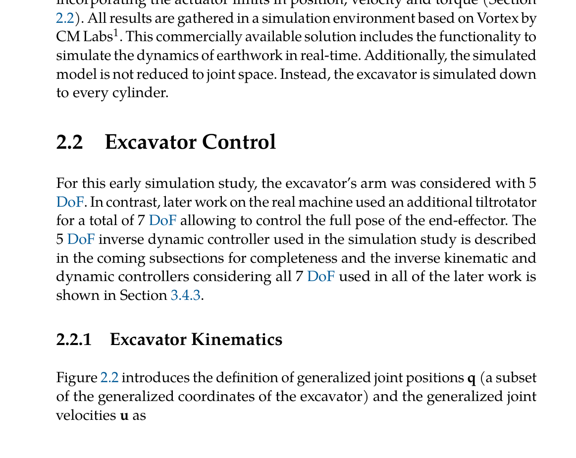
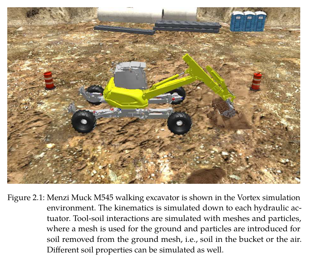
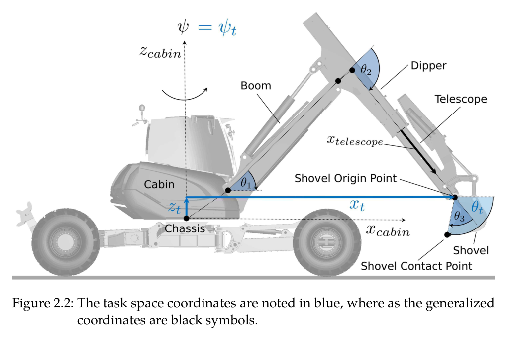
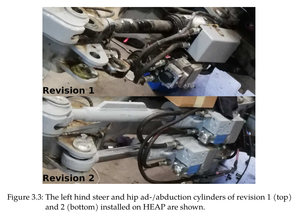
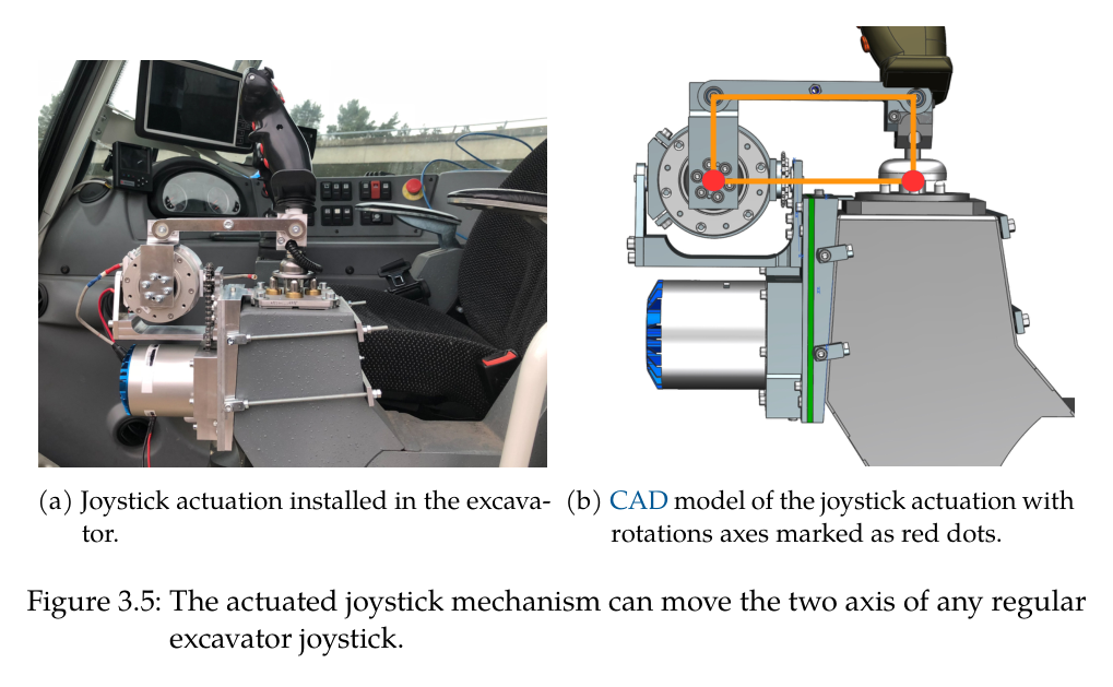
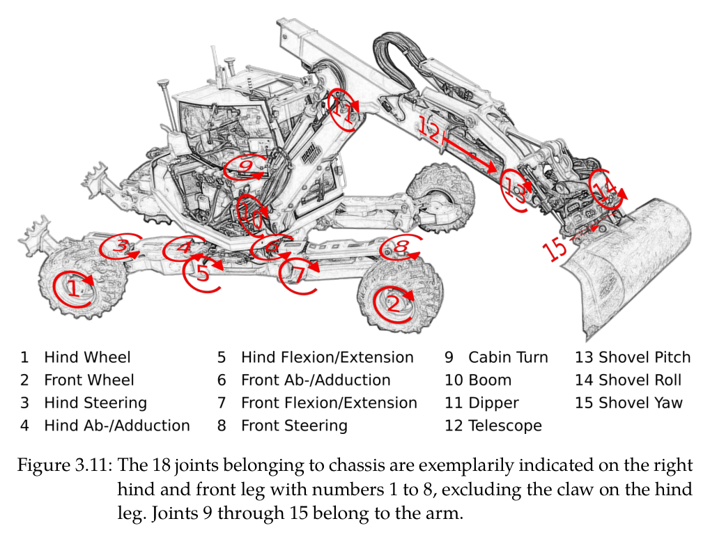
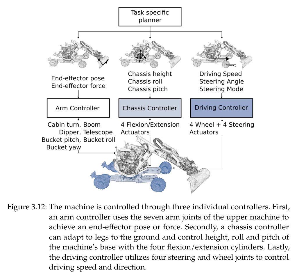
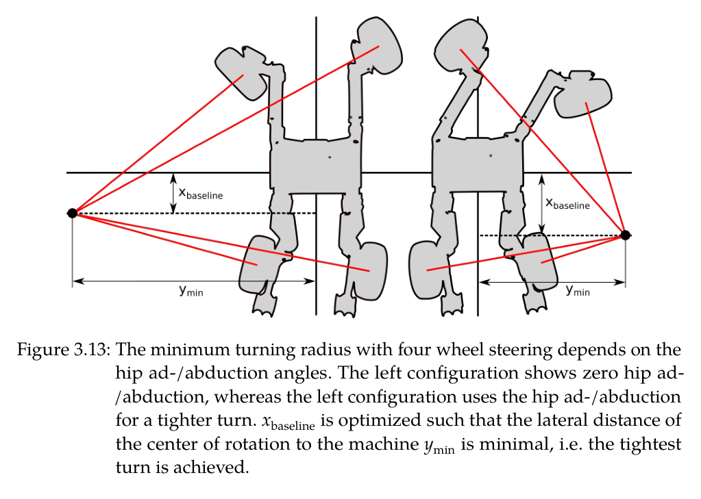
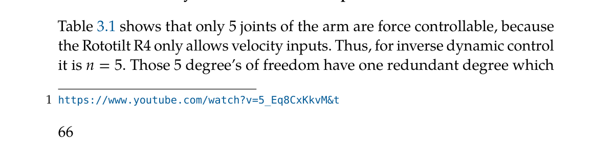
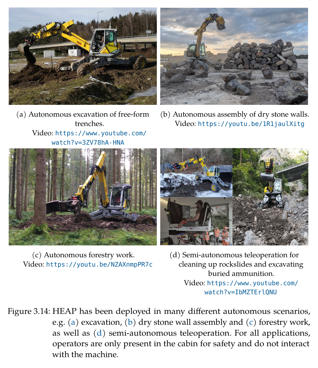
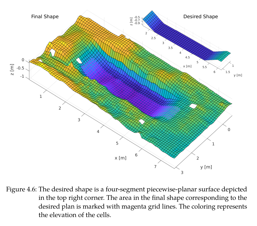
원문 Figure 2.2 · PDF p.34 — Figure 2.2 introduces the definition of generalized joint positions 𝐪(a subset of the generalized coordinates of the excavator) and the generalized joint velocities 𝐮as원문 Figure 2.1 · PDF p.35 — Figure 2.1: Menzi Muck M545 walking excavator is shown in the Vortex simulation environment. The kinematics is simulated down to each hydraulic ac- tuator. Tool-soil interactions are simulated with meshes and particles, where a mesh is used for the ground and particles are introduced for soil removed from the ground mesh, i.e., soil in the bucket or the air. Different soil properties can be simulated as well.원문 Figure 2.2 · PDF p.36 — Figure 2.2: The task space coordinates are noted in blue, where as the generalized coordinates are black symbols.원문 Figure 2.3 · PDF p.40 — Figure 2.3: The different phases of a dig cycle in chronological order from left to right.원문 Figure 2.7 · PDF p.46 — Figure 2.7: Illustration of finding the point of attack. Solid line: desired elevation. Dashed line: desired elevation with an added threshold 𝜃+. Black line: actual terrain elevation. Black dashed line: Rough guess of the removed material for illustration purposes. Orange point: chosen point of attack. Blue line: Imaginary planning line. Blue arrow: Working direction. 𝛼: Maximum slope. 𝑣offset: Vertical offset of the PoA원문 Figure 2.8 · PDF p.47 — Figure 2.8: Illustration of finding the dump point. Solid line: Desired elevation. Dashed line: Desired elevation with a substracted threshold 𝜃−. Black line: Actual terrain elevation. Black dashed line: Rough guess of the added material for illustration purposes. Orange point: Chosen dump point. Blue line: Imaginary planning line. Blue arrow: Working direction. 𝛼: Maximum slope. ℎoffset: Height offset of the dumping point.원문 Table 2.1 · PDF p.48 — Table 2.1: The chosen design parameter values for the excavation planning and control are shown.원문 Figure 2.10 · PDF p.50 — Figure 2.10: The three different phases during a single dig cycle are shown. 1: Pen- etrate. 2: Drag. 3: Close. The solid blue line is the x-z-trajectory of the shovel origin, whereas the blue dashed line is the shovel edge. The black dashed line connects the shovel edge and origin when the phase changes.원문 Figure 2.11 · PDF p.51 — Figure 2.11: Digging in soft clay (red dotted line) shows a different trajectory than digging in harder loam (blue dotted line). Both trajectories represent the motion of the shovel edge in x-z-coordinates in task space. The black line is the ground level prior to the dig.원문 Figure 2.5 · PDF p.51 — Figure 2.5 shows a simple example with an actual terrain and the desired terrain illustrated as the gray striped area. Let us assume that the point of attack is at the position where the shovel is shown in Figure 2.5. The force trajectory, which is then applied to the shovel to execute a single dig cycle, is plotted in Figure 2.12 (solid lines), together with an uninfluenced force trajectory (dashed lines). The point of attack is already very close to the원문 Figure 2.12 · PDF p.52 — Figure 2.12: The prototype force trajectory in x and z (dashed lines) is compared to the adjusted force trajectory (solid lines) when the shovel is close to a desired shape as shown in Figure 2.5.원문 Figure 2.15 · PDF p.54 — Figure 2.15: The error volume is plotted over the number of dig cycles for the linear trench as well as the curved trench. The bend indicates the transition to the refinement steps.원문 Figure 3.1 · PDF p.58 — Figure 3.1: HEAP, the first of its kind for autonomous deployment, in front of its clone Armano, a proof of concept for teleoperated/semi-autonomous operation.원문 Table 3.1 · PDF p.60 — Table 3.1: HEAP’s different joints have different capabilities. This table provides an overview of the possible measurements and realized actuation principles per joint. ✓/✗marks available/unavailable feedback or actuation. ✓in- dicates for the wheels that the velocity cannot be measured directly, but instead, it can be estimated from the chassis’ linear velocity.원문 Figure 3.3 · PDF p.61 — Figure 3.3: The left hind steer and hip ad-/abduction cylinders of revision 1 (top) and 2 (bottom) installed on HEAP are shown.원문 Figure 3.4 · PDF p.62 — Figure 3.4 shows the level of intrusion of these three different principles. Whereas the actuated joystick (orange) is minimally invasive and requires no tampering with the existing hydraulics (black), the pilot stage valves (blue) require the hydraulic low-pressure circuit and the servo valves (red) in order for the high-pressure circuit to be opened. The pre-installed main stage and the servo valves are supplied by two different pump systems. The main stage uses a traditional load sensing system that only raises the system원문 Figure 3.4 · PDF p.63 — Figure 3.4: The three different actuation types are joystick actuation (orange), elec- tric pilot stage valves (blue) and Moog servo valves (red). The black lines and boxes represent the standard components already installed by the machine manufacturer. Note that a different pump is used for the servo valve as for the main stage valves. This second pump is normally used to supply large hydraulic attachments.원문 Figure 3.5 · PDF p.64 — Figure 3.5: The actuated joystick mechanism can move the two axis of any regular excavator joystick.원문 Figure 3.6 · PDF p.66 — Figure 3.6: The servo valves for boom, dipper, telescope and shovel joint together with the encapsulated accumulator in the supply line (on the left) are located next to the operator’s cabin.원문 Figure 3.7 · PDF p.67 — Figure 3.7: Velocity control comparison of servo valve (orange), pilot stage valve (blue) and actuated joystick (yellow) on the boom (solid line), dipper (dashed line) and shovel (dotted line) cylinder.원문 Table 3.2 · PDF p.68 — Table 3.2: The velocity control performance is evaluated by measuring the 𝑡90 time and the cut-off frequency.원문 Table 3.3 · PDF p.69 — Table 3.3: The force control performance is evaluated by measuring the 𝑡90 time and the cut-off frequency.원문 Figure 3.8 · PDF p.70 — Figure 3.8: Force control comparison of servo valve (orange), pilot stage valve (blue) and actuated joystick (yellow) on the boom (solid line), dipper (dashed line) and shovel (dotted line) cylinder.원문 Figure 3.9 · PDF p.72 — Figure 3.9: An experiment, where the maximum current is applied to the pilot stage valve, reveals the partition of the overall delay of 380ms to 60ms of the pilot stage and 320ms of the main valves.원문 Figure 3.10 · PDF p.77 — Figure 3.10: The sum of squared errors in orientation is depicted in the upper plot and for the position in the lower plot. The estimator is initialized with unknown biases at time 0s and the machine stays stationary until time 12s, where it then starts to move the legs and drive. The IMU/GNSS approach (solid line) shows higher initial errors, but outperforms the IMU/GNSS/Roll/Leg approach (dashed line) once the machine starts to move.원문 Figure 3.11 · PDF p.79 — Figure 3.11: The 18 joints belonging to chassis are exemplarily indicated on the right hind and front leg with numbers 1 to 8, excluding the claw on the hind leg. Joints 9 through 15 belong to the arm.원문 Figure 3.12 · PDF p.80 — Figure 3.12: The machine is controlled through three individual controllers. First, an arm controller uses the seven arm joints of the upper machine to achieve an end-effector pose or force. Secondly, a chassis controller can adapt to legs to the ground and control height, roll and pitch of the machine’s base with the four flexion/extension cylinders. Lastly, the driving controller utilizes four steering and wheel joints to control driving speed and direction.원문 Figure 3.13 · PDF p.81 — Figure 3.13: The minimum turning radius with four wheel steering depends on the hip ad-/abduction angles. The left configuration shows zero hip ad- /abduction, whereas the left configuration uses the hip ad-/abduction for a tighter turn. 𝑥baseline is optimized such that the lateral distance of the center of rotation to the machine 𝑦min is minimal, i.e. the tightest turn is achieved.원문 Table 3.1 · PDF p.82 — Table 3.1 shows that only 5 joints of the arm are force controllable, because the Rototilt R4 only allows velocity inputs. Thus, for inverse dynamic control it is 𝑛= 5. Those 5 degree’s of freedom have one redundant degree which원문 Figure 3.14 · PDF p.88 — Figure 3.14: HEAP has been deployed in many different autonomous scenarios, e.g. (a) excavation, (b) dry stone wall assembly and (c) forestry work, as well as (d) semi-autonomous teleoperation. For all applications, operators are only present in the cabin for safety and do not interact with the machine.원문 Figure 4 · PDF p.101 — Figure 4.7a원문 Figure 4 · PDF p.101 — Figure 4.7b원문 Figure 4 · PDF p.101 — Figure 4.7c원문 Figure 4.6 · PDF p.103 — Figure 4.6: The desired shape is a four-segment piecewise-planar surface depicted in the top right corner. The area in the final shape corresponding to the desired plan is marked with magenta grid lines. The coloring represents the elevation of the cells.원문 Figure 4.7 · PDF p.105 — Figure 4.7 explains in detail the process of autonomous excavation on the example of the 9th, 12th and 13th dig cycle. Note that there are two dig cycles between Figure 4.7a and 4.7b that are not shown in this sequence. The corresponding decisions taken in the state machine for these three individual dig cycles is illustrated in Figure 4.5 with colored lines. The excavator is positioned to the left of the plots and works from right to left. First, in Figure 4.7a, the planned point of attack is already close to the desired surface. Thus, the bucket tries to track the desired surface as close as possible with the servo valves and the inverse kinematic controller until the estimated contact force exceeds a threshold. The state machine then switches to force controlled digging to fill the bucket despite large interaction forces. The excavation planner chooses the point of attack for the excavation such that it does not excavate at the very bottom of a steep wall. The arm could collide with the top edge of the trench and the forces at the bottom of such a steep wall would prevent successful excavation. Figure 4.7b shows such a dig cycle were the planner chooses a point not at the bottom of the trench to first remove the soil on top. The point of attack is not close to the desired shape. Thus the digging cycle is fully force- controlled without forcing the bucket to stay on a certain trajectory. The bucket trajectory results from applying the force trajectory and how the soil reacts to this applied force. Thus, it is only a coincidence that the bucket trajectory in Figure 4.7b is a straight and horizontal line. With the pile of soil removed from the previous dig cycle, the bucket is filled in the cycle in Figure 4.7c only by tracking the desired shape as there is only very little soil left in that part of the trench. The shape error of the finished trench is shown in Figure 4.8 before and after autonomous excavation. It shows a cut through the trench in longi- tudinal (x-)direction. The error bars represent the average error in lateral (y-)direction. The four-segment piecewise-planar shape was excavated with a mean error of 0.027m and a standard deviation of 0.035m. Figure 4.8 shows additionally the 𝜎-error bound. Note that this approach shows the same accuracy for horizontal planes as well as angled slopes. Additionally, the approach was also tested on a free-form curved shape shown in Figure 4.9. The shape was successfully excavated with a mean error of 0.024m and a standard deviation of 0.032m. Figure 4.8 and 4.9 in combination show that free-form shapes can be excavated with this approach with unprecedented high accuracy. The results shown in this chapter are compared to our previous work in simulation in Chapter 2, Shao et al. [62] and Maeda et al. [12]. In our원문 Figure 5.3 · PDF p.114 — Figure 5.3: The location where experiments are conducted is shown in the large 3D point cloud gathered by the drone and consisting of 17 million points. The test field in the white rectangle is converted into a 2.5D elevation map for use in the design environment.원문 Figure 5.4 · PDF p.115 — Figure 5.4: The robotic embankment design is created on the elevation map gathered with the mapping drone.원문 Figure 5.7 · PDF p.120 — Figure 5.7: In order to achieve a clear break line between the swale and front face, the bucket has to pass over it with a parallel bucket edge meaning that the working direction of the bucket is orthogonal to the design line.원문 Figure 5.12 · PDF p.126 — Figure 5.12: An elevation map of the s-curved embankment is created from the on-board LiDAR’s after the experiment was successfully finished. The colors represent the terrain height.원문 Figure 5.14 · PDF p.128 — Figure 5.14: The swale, to catch water runoff, and the front face are functional parts that should not be changed. The embankment volume can still be adapted to compensate an offset in cut and fill volumes by dropping the ridgeline along the front face. This will remove a large volume (black and white stripes) at the backside of the embankment. This is illustrated through a section cut at the point with the biggest correction.원문 Figure 5.15 · PDF p.129 — Figure 5.15: The two-faced embankment with a corner is defined by a CAD model designed in Blender.원문 Table 6.1 · PDF p.134 — Table 6.1: The average errors per grid cell of all excavation experiments are com- pared in this table. It shows that the advances from simulation transfer to reality without additional error and more complex designs can also be achieved with high precision.